The use of machine learning methods on time series data requires feature engineering.
A univariate time series dataset is only comprised of a sequence of observations. These must be transformed into input and output features in order to use supervised learning algorithms.
The problem is that there is little limit to the type and number of features you can engineer for a time series problem. Classical time series analysis tools like the correlogram can help with evaluating lag variables, but do not directly help when selecting other types of features, such as those derived from the timestamps (year, month or day) and moving statistics, like a moving average.
In this tutorial, you will discover how you can use the machine learning tools of feature importance and feature selection when working with time series data.
After completing this tutorial, you will know:
- How to create and interpret a correlogram of lagged observations.
- How to calculate and interpret feature importance scores for time series features.
- How to perform feature selection on time series input variables.
Kick-start your project with my new book Time Series Forecasting With Python, including step-by-step tutorials and the Python source code files for all examples.
Let’s get started.
- Updated Apr/2019: Updated the link to dataset.
- Updated Jun/2019: Fixed indenting.
- Updated Aug/2019: Updated data loading to use new API.
- Updated Sep/2020: Updated code to match changes to the API.
Tutorial Overview
This tutorial is broken down into the following 5 steps:
- Monthly Car Sales Dataset: That describes the dataset we will be working with.
- Make Stationary: That describes how to make the dataset stationary for analysis and forecasting.
- Autocorrelation Plot: That describes how to create a correlogram of the time series data.
- Feature Importance of Lag Variables: That describes how to calculate and review feature importance scores for time series data.
- Feature Selection of Lag Variables: That describes how to calculate and review feature selection results for time series data.
Let’s start off by looking at a standard time series dataset.
Stop learning Time Series Forecasting the slow way!
Take my free 7-day email course and discover how to get started (with sample code).
Click to sign-up and also get a free PDF Ebook version of the course.
Monthly Car Sales Dataset
In this tutorial, we will use the Monthly Car Sales dataset.
This dataset describes the number of car sales in Quebec, Canada between 1960 and 1968.
The units are a count of the number of sales and there are 108 observations. The source data is credited to Abraham and Ledolter (1983).
Download the dataset and save it into your current working directory with the filename “car-sales.csv“. Note, you may need to delete the footer information from the file.
The code below loads the dataset as a Pandas Series object.
|
1 2 3 4 5 6 7 8 9 10 |
# line plot of time series from pandas import read_csv from matplotlib import pyplot # load dataset series = read_csv('car-sales.csv', header=0, index_col=0) # display first few rows print(series.head(5)) # line plot of dataset series.plot() pyplot.show() |
Running the example prints the first 5 rows of data.
|
1 2 3 4 5 6 7 |
Month 1960-01-01 6550 1960-02-01 8728 1960-03-01 12026 1960-04-01 14395 1960-05-01 14587 Name: Sales, dtype: int64 |
A line plot of the data is also provided.
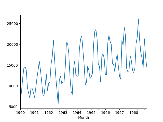
Monthly Car Sales Dataset Line Plot
Make Stationary
We can see a clear seasonality and increasing trend in the data.
The trend and seasonality are fixed components that can be added to any prediction we make. They are useful, but need to be removed in order to explore any other systematic signals that can help make predictions.
A time series with seasonality and trend removed is called stationary.
To remove the seasonality, we can take the seasonal difference, resulting in a so-called seasonally adjusted time series.
The period of the seasonality appears to be one year (12 months). The code below calculates the seasonally adjusted time series and saves it to the file “seasonally-adjusted.csv“.
|
1 2 3 4 5 6 7 8 9 10 11 12 13 14 |
# seasonally adjust the time series from pandas import read_csv from matplotlib import pyplot # load dataset series = read_csv('car-sales.csv', header=0, index_col=0) # seasonal difference differenced = series.diff(12) # trim off the first year of empty data differenced = differenced[12:] # save differenced dataset to file differenced.to_csv('seasonally_adjusted.csv', index=False) # plot differenced dataset differenced.plot() pyplot.show() |
Because the first 12 months of data have no prior data to be differenced against, they must be discarded.
The stationary data is stored in “seasonally-adjusted.csv“. A line plot of the differenced data is created.
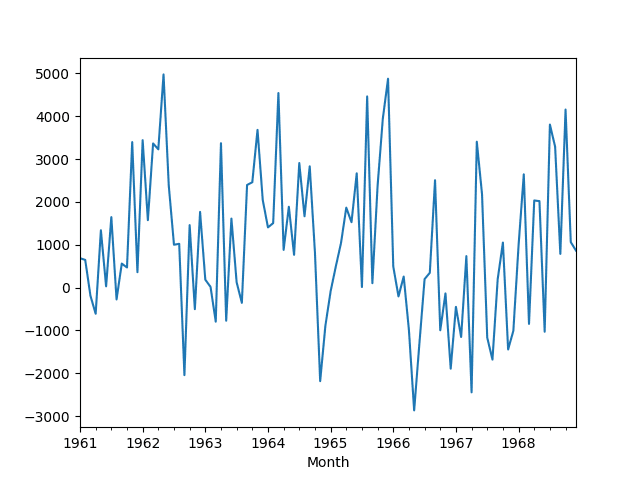
Seasonally Differenced Monthly Car Sales Dataset Line Plot
The plot suggests that the seasonality and trend information was removed by differencing.
Autocorrelation Plot
Traditionally, time series features are selected based on their correlation with the output variable.
This is called autocorrelation and involves plotting autocorrelation plots, also called a correlogram. These show the correlation of each lagged observation and whether or not the correlation is statistically significant.
For example, the code below plots the correlogram for all lag variables in the Monthly Car Sales dataset.
|
1 2 3 4 5 6 |
from pandas import read_csv from statsmodels.graphics.tsaplots import plot_acf from matplotlib import pyplot series = read_csv('seasonally_adjusted.csv', header=0) plot_acf(series) pyplot.show() |
Running the example creates a correlogram, or Autocorrelation Function (ACF) plot, of the data.
The plot shows lag values along the x-axis and correlation on the y-axis between -1 and 1 for negatively and positively correlated lags respectively.
The dots above the blue area indicate statistical significance. The correlation of 1 for the lag value of 0 indicates 100% positive correlation of an observation with itself.
The plot shows significant lag values at 1, 2, 12, and 17 months.
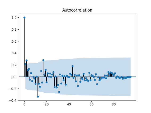
Correlogram of the Monthly Car Sales Dataset
This analysis provides a good baseline for comparison.
Time Series to Supervised Learning
We can convert the univariate Monthly Car Sales dataset into a supervised learning problem by taking the lag observation (e.g. t-1) as inputs and using the current observation (t) as the output variable.
We can do this in Pandas using the shift function to create new columns of shifted observations.
The example below creates a new time series with 12 months of lag values to predict the current observation.
The shift of 12 months means that the first 12 rows of data are unusable as they contain NaN values.
|
1 2 3 4 5 6 7 8 9 10 11 12 13 |
from pandas import read_csv from pandas import DataFrame # load dataset series = read_csv('seasonally_adjusted.csv', header=0) # reframe as supervised learning dataframe = DataFrame() for i in range(12,0,-1): dataframe['t-'+str(i)] = series.shift(i).values[:,0] dataframe['t'] = series.values[:,0] print(dataframe.head(13)) dataframe = dataframe[13:] # save to new file dataframe.to_csv('lags_12months_features.csv', index=False) |
Running the example prints the first 13 rows of data showing the unusable first 12 rows and the usable 13th row.
|
1 2 3 4 5 6 7 8 9 10 11 12 13 14 15 16 17 18 19 20 21 22 23 24 25 26 27 28 29 |
t-12 t-11 t-10 t-9 t-8 t-7 t-6 t-5 \ 1961-01-01 NaN NaN NaN NaN NaN NaN NaN NaN 1961-02-01 NaN NaN NaN NaN NaN NaN NaN NaN 1961-03-01 NaN NaN NaN NaN NaN NaN NaN NaN 1961-04-01 NaN NaN NaN NaN NaN NaN NaN NaN 1961-05-01 NaN NaN NaN NaN NaN NaN NaN NaN 1961-06-01 NaN NaN NaN NaN NaN NaN NaN 687.0 1961-07-01 NaN NaN NaN NaN NaN NaN 687.0 646.0 1961-08-01 NaN NaN NaN NaN NaN 687.0 646.0 -189.0 1961-09-01 NaN NaN NaN NaN 687.0 646.0 -189.0 -611.0 1961-10-01 NaN NaN NaN 687.0 646.0 -189.0 -611.0 1339.0 1961-11-01 NaN NaN 687.0 646.0 -189.0 -611.0 1339.0 30.0 1961-12-01 NaN 687.0 646.0 -189.0 -611.0 1339.0 30.0 1645.0 1962-01-01 687.0 646.0 -189.0 -611.0 1339.0 30.0 1645.0 -276.0 t-4 t-3 t-2 t-1 t 1961-01-01 NaN NaN NaN NaN 687.0 1961-02-01 NaN NaN NaN 687.0 646.0 1961-03-01 NaN NaN 687.0 646.0 -189.0 1961-04-01 NaN 687.0 646.0 -189.0 -611.0 1961-05-01 687.0 646.0 -189.0 -611.0 1339.0 1961-06-01 646.0 -189.0 -611.0 1339.0 30.0 1961-07-01 -189.0 -611.0 1339.0 30.0 1645.0 1961-08-01 -611.0 1339.0 30.0 1645.0 -276.0 1961-09-01 1339.0 30.0 1645.0 -276.0 561.0 1961-10-01 30.0 1645.0 -276.0 561.0 470.0 1961-11-01 1645.0 -276.0 561.0 470.0 3395.0 1961-12-01 -276.0 561.0 470.0 3395.0 360.0 1962-01-01 561.0 470.0 3395.0 360.0 3440.0 |
The first 12 rows are removed from the new dataset and results are saved in the file “lags_12months_features.csv“.
This process can be repeated with an arbitrary number of time steps, such as 6 months or 24 months, and I would recommend experimenting.
Feature Importance of Lag Variables
Ensembles of decision trees, like bagged trees, random forest, and extra trees, can be used to calculate a feature importance score.
This is common in machine learning to estimate the relative usefulness of input features when developing predictive models.
We can use feature importance to help to estimate the relative importance of contrived input features for time series forecasting.
This is important because we can contrive not only the lag observation features above, but also features based on the timestamp of observations, rolling statistics, and much more. Feature importance is one method to help sort out what might be more useful in when modeling.
The example below loads the supervised learning view of the dataset created in the previous section, fits a random forest model (RandomForestRegressor), and summarizes the relative feature importance scores for each of the 12 lag observations.
A large-ish number of trees is used to ensure the scores are somewhat stable. Additionally, the random number seed is initialized to ensure that the same result is achieved each time the code is run.
|
1 2 3 4 5 6 7 8 9 10 11 12 13 14 15 16 17 18 19 20 |
from pandas import read_csv from sklearn.ensemble import RandomForestRegressor from matplotlib import pyplot # load data dataframe = read_csv('lags_12months_features.csv', header=0) array = dataframe.values # split into input and output X = array[:,0:-1] y = array[:,-1] # fit random forest model model = RandomForestRegressor(n_estimators=500, random_state=1) model.fit(X, y) # show importance scores print(model.feature_importances_) # plot importance scores names = dataframe.columns.values[0:-1] ticks = [i for i in range(len(names))] pyplot.bar(ticks, model.feature_importances_) pyplot.xticks(ticks, names) pyplot.show() |
Running the example first prints the importance scores of the lagged observations.
|
1 2 |
[ 0.21642244 0.06271259 0.05662302 0.05543768 0.07155573 0.08478599 0.07699371 0.05366735 0.1033234 0.04897883 0.1066669 0.06283236] |
The scores are then plotted as a bar graph.
The plot shows the high relative importance of the observation at t-12 and, to a lesser degree, the importance of observations at t-2 and t-4.
It is interesting to note a difference with the outcome from the correlogram above.
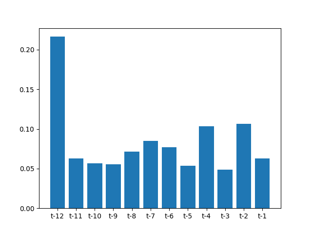
Bar Graph of Feature Importance Scores on the Monthly Car Sales Dataset
This process can be repeated with different methods that can calculate importance scores, such as gradient boosting, extra trees, and bagged decision trees.
Feature Selection of Lag Variables
We can also use feature selection to automatically identify and select those input features that are most predictive.
A popular method for feature selection is called Recursive Feature Selection (RFE).
RFE works by creating predictive models, weighting features, and pruning those with the smallest weights, then repeating the process until a desired number of features are left.
The example below uses RFE with a random forest predictive model and sets the desired number of input features to 4.
|
1 2 3 4 5 6 7 8 9 10 11 12 13 14 15 16 17 18 19 20 21 22 23 24 25 |
from pandas import read_csv from sklearn.feature_selection import RFE from sklearn.ensemble import RandomForestRegressor from matplotlib import pyplot # load dataset dataframe = read_csv('lags_12months_features.csv', header=0) # separate into input and output variables array = dataframe.values X = array[:,0:-1] y = array[:,-1] # perform feature selection rfe = RFE(RandomForestRegressor(n_estimators=500, random_state=1), n_features_to_select=4) fit = rfe.fit(X, y) # report selected features print('Selected Features:') names = dataframe.columns.values[0:-1] for i in range(len(fit.support_)): if fit.support_[i]: print(names[i]) # plot feature rank names = dataframe.columns.values[0:-1] ticks = [i for i in range(len(names))] pyplot.bar(ticks, fit.ranking_) pyplot.xticks(ticks, names) pyplot.show() |
Running the example prints the names of the 4 selected features.
Unsurprisingly, the results match features that showed a high importance in the previous section.
|
1 2 3 4 5 |
Selected Features: t-12 t-6 t-4 t-2 |
A bar graph is also created showing the feature selection rank (smaller is better) for each input feature.
Bar Graph of Feature Selection Rank on the Monthly Car Sales Dataset
This process can be repeated with different numbers of features to select more than 4 and different models other than random forest.
Summary
In this tutorial, you discovered how to use the tools of applied machine learning to help select features from time series data when forecasting.
Specifically, you learned:
- How to interpret a correlogram for highly correlated lagged observations.
- How to calculate and review feature importance scores in time series data.
- How to use feature selection to identify the most relevant input variables in time series data.
Do you have any questions about feature selection with time series data?
Ask your questions in the comments and I will do my best to answer.
Want to Develop Time Series Forecasts with Python?

Develop Your Own Forecasts in Minutes
...with just a few lines of python codeDiscover how in my new Ebook:
Introduction to Time Series Forecasting With Python
It covers self-study tutorials and end-to-end projects on topics like: Loading data, visualization, modeling, algorithm tuning, and much more...
Finally Bring Time Series Forecasting to
Your Own Projects
Skip the Academics. Just Results.


Hi Jason big fan! I was wondering if you are going to a series on multivariate array time series forecasting.
Many thanks,
Best,
Andrew
Yes, I hope to cover this soon Andrew.
Please have you done this? Feature Selection for multivariate Time Series Forecasting
I don’t have a tutorial on this topic, sorry.
Hello Jason,
Many thanks for this blog. I will be so Interested to see how the multivariate Time Series Forecast is dealt with.
Keep up the good works,
Best Regards
Ben
Thanks Ben, I hope to cover multivariate time series soon.
Hello, great work, Looking Forward to this…do you have an estimate of how soon
Yes, I have many examples here:
https://machinelearningmastery.com/start-here/#deep_learning_time_series
Hello Jason,
I wondered about your choice to keep only the last 12 lags for the feature importance and feature selection study.
Because i understand the correlogram showed you should push the study until the 17 lag (correlogram showed 1, 2, 12, and 17 lags are correlated to current state)
I m I right?
Thanks for your work!
Yes, I kept it short for brevity.
The output of this lines
‘plot_acf(series)’
‘pyplot.show()’
is not like yours. It just shows an straight line.
May you please check it.
Thanks
Yeah, the plot_acf thing is not working properly.
What problem do you see exactly?
What version of statsmodels are you using?
I can confirm the example, please check that you have all of the code and the same source data.
I had a similar issue. It is due to the footer if you do not delete in the data set or drop the last row in the series after import.
Hello Jason!
Can you recommend some references about recursive feature selection and random forest on feature selection for time series?
Thanks!
No. My best advice: try it, get results and use them in developing better models.
Hi Jason!
I am still unable to understand the importance of lag variable?
Is lag applied to a feature variable to find correlation with the target variable?
Thanks!
A lag is a past observation, an observation at a prior time step.
We can use these as input features to learning models. So abstractly we can predict today based on what happened yesterday.
Yesterday’s ob is a lag variable.
Does that help?
Dear Jason,
I am trying to run your code above with X size of (358,168) and test y (358,24), and having error “ValueError: bad input shape (358, 24)”. I would like to find the most relevant 12 features from 168 features in X(358,168) depending on 24 output of y(358,24)
My y matrix has 24 output instead of 1. What might be the reason for the error?
X = array[:,0:168]
y = array[:,168:192]
rfe = RFE(RandomForestRegressor(n_estimators=500, random_state=1), 12)
fit = rfe.fit(X, y)
That might be too many output variables, most algorithms expect a single output variable in sklearn.
I can’t think of any that support multiple, but I could be wrong.
You might like to explore a neural network model instead?
Thanks for your comment Jason.
Actually, what I would like to do is determining the most relevant feature with RFE, then training a neural network model with this features. Do you think it is a reasonable approach?
For the multiple output error, I will run RFE for each output instead of 24 one by one.
You could try it and it would make sense if there is one highly predictive feature, but I would encourage you to test many configurations.
Thanks for the great tutorial.
I was wondering if you could explain the logic of why ACF might show some lags as statistically significant, while feature selection might show totally different lags as having predictive power.
Different operate under different assumptions and in turn, produce differing results. This is to be expected.
hello Jason,
Thank you for the post loved it!
I’m a bit confused about the following:
“This is important because we can contrive not only the lag observation features above, but also features based on the timestamp of observations, rolling statistics, and much more.”
Would it make sense for me to add “month” to the set of features(“X”) if I have removed the seasonality from the time series already? Also, about the “much more” part, does stationarity still mean anything if I add extra features to “X”?
If it is not a problem, why do we require the data to be stationary in the first place?
If it is a problem, how do we make sure that the data is still stationary after we add extra features to “X”?
Yes, but you can also explore non-linear methods that offer more flexibility when it comes to stationarity requirements.
Great tutorial! I have moderate experience with time series data. I am into detecting the most important features for a time series financial data for a binary classification task. And I have about 400 features (many of them highly correlated after I make the data stationary). How could I apply the method you show above? Getting the let’s say 10 previous days for each feature? Or do you have other suggestions?
Thanks in advance!
I would recommend exploring a suite of approaches and see what features result in the best model skill.
Hi Jason,
This is great! How would you go about feature selection for time series using LSTM/keras. In that case, there won’t be a need to deconstruct the time series into the different lag variables from t to t-12.
I’m currently working on a time series problem with multiple predictors. I need to know which predictors are important. Is the process the same as what you would do here or can I use a randomforest’s importance feature?
Thanks!
Good question.
There may be specialised methods, but I’m not across them right now – perhaps do a little research.
I’d suggest grid searching models across different subsets of features to see what is important/results in better model skill. Basically an RFE approach.
Hi Jason,
I’m assuming we can extend this feature importance and selection beyond lag variables:
– “temporal/seasonal features” such is hour of day,month of year etc
– external variables that depend on the problem
– rolling features such as min, max and mean of value of temperature in this case over past n days for example
Essentially the features you provided in link below, we can then perfrom feature importance and selection, would you agree?
https://machinelearningmastery.com/basic-feature-engineering-time-series-data-python/
Sure. I don’t have a lot of material on multivaraite time series though, I hope to cover it more in the future.
Am i right in saying the process of feature selection/importance/etc occurs AFTER fitting the model to the training data?
Features should be chosen prior to fitting a model.
Note though that the process of working through is iterative. Lots of looping back to prior steps.
the observations in your training data are not iid. Do you think it is ok for your model?
Making the series stationary removes the time dependence.
RandomForestRegressor does bootstrap. Would not this be data leakage considering that the example is a time series?
How so?
Here’s a better explanation:
https://stats.stackexchange.com/questions/25706/how-do-you-do-bootstrapping-with-time-series-data
Hi, Jason
I am using RandomForest for forecasting rainfall variable. I have around 15 predictors with 50 years data. When I am predicting rainfall values based on the predictors (variables), I am getting very low values as compared to original rainfalls. I mean, I am totally missing extreme values. Please suggest.
Regards,
Vishu
I have some suggestions here:
https://machinelearningmastery.com/machine-learning-performance-improvement-cheat-sheet/
Hi Jason,
Thanks for the blog. I learned a lot thanks to you.
I’m looking for a method of selecting variables for time series like the RFE. But after reading this new post (https://machinelearningmastery.com/how-to-predict-whether-eyes-are-open-or-closed-using-brain-waves/), I have doubts about whether it is possible to apply a method that uses bootstrap.
I think that when using RFE, the evaluation of the models does not respect the temporal ordering of the observations, as it happens in your post about how to predict whether eyes are open or closed and that uses the future information for the selection of variables. What do you think? Thanks!!
Regards
It is a challenge. You could try classical feature selection methods, like RFE and correlation, knowing there is bias, then build models from the suggestions and compare the performance to using all features.
Hi Jason,
Many thanks for this blog.
I use Simple Linear Regression in Sklearn.
I have this error (could not convert to float: ‘(TOP (S (S (NP *’)
I think it’s ncessary to encod categorical data !!!
But, my dateset is for natural language processing (data from conll-2012).
I use another algorithm that accepts string variables or there are an other solution?
I explain how to work with text data here:
https://machinelearningmastery.com/start-here/#nlp
Thank you 🙂
Hi Jason,
Thank you for your great tutorials.
Unfortunately, I got a problem running the code. The result of the code on my computer is exactly the same as yours till Autocorrelation Plot. At Autocorrelation Plot, my result just shows a straight line at zero.
The next, there is an error as follows.
runfile(‘C:/Users/Hossein/.spyder-py3/temp.py’, wdir=’C:/Users/Hossein/.spyder-py3′)
Traceback (most recent call last):
File “C:\Users\Hossein\Anaconda3\lib\site-packages\IPython\core\interactiveshell.py”, line 2862, in run_code
exec(code_obj, self.user_global_ns, self.user_ns)
File “”, line 1, in
runfile(‘C:/Users/Hossein/.spyder-py3/temp.py’, wdir=’C:/Users/Hossein/.spyder-py3′)
File “C:\Users\Hossein\Anaconda3\lib\site-packages\spyder\utils\site\sitecustomize.py”, line 705, in runfile
execfile(filename, namespace)
File “C:\Users\Hossein\Anaconda3\lib\site-packages\spyder\utils\site\sitecustomize.py”, line 102, in execfile
exec(compile(f.read(), filename, ‘exec’), namespace)
File “C:/Users/Hossein/.spyder-py3/temp.py”, line 48
dataframe[‘t-‘+str(i)] = series.shift(i)
^
IndentationError: expected an indented block
Looks like you did not copy the code with the indenting, here’s how to copy code:
https://machinelearningmastery.com/faq/single-faq/how-do-i-copy-code-from-a-tutorial
Also, I recommend running code from the command line:
https://machinelearningmastery.com/faq/single-faq/how-do-i-run-a-script-from-the-command-line
Thank you for your prompt response.
Unfortunately, I still have the same problem. Even I tried your code on https://repl.it and it showed the same error.
dataframe[‘t-‘+str(i)] = series.shift(i)
^
IndentationError: expected an indented block
Perhaps try copy-pasting the code again and indenting it manually in your text editor?
Looks to me that when you yourself pasted the code it did not properly indent, because the box doesn’t show any kind of indentation (might also be a problem to do with the website or the browser, do you see any indentation on the code box?).
thanks for the tutorial, good stuff
You’re right, I have added indenting to the example.
Sorry about that.
I figured it out, finally.
The autocorrelation plot doesn’t show since there are two “nan”s at the end of series.
add “series=series[1:-2]” after reading the following line.
series = Series.from_csv(‘seasonally_adjusted.csv’, header=None)
Another comment regarding the error in Time Series to Supervised Learning.
the code needs a space just after “for” loop as follows:
for i in range(12,0,-1):
dataframe[‘t-‘+str(i)] = series.shift(i)
Codes don’t work. I get length of values does not match length of index, when you creating the dataframe with the shifted columns. I don’t know how could you produce the results with this code.
Sorry to hear that, I have some suggestions for you here:
https://machinelearningmastery.com/faq/single-faq/why-does-the-code-in-the-tutorial-not-work-for-me
Hi Jason,
I’m struggling a bit to understand the feature importance and selection results. Specifically, how is it possible for lag t-12 to have such a high impact in predicting the time series after having removed the seasonality of 12 month in the differencing step before?
Perhaps the seasonal correction did not remove all of the seasonal structure.
Hello Jason,
Thanks for the article!
The time series I have is daily data of 4 years and 10 months.
I am actually implementing SARIMAX for my time series data and I am including several exogenous variables.
I actually did the feature selection you explained above on the exogenous variables and also on 10 lags.
I included in my exogenous variables the mean of my time series over the year (so 364 value where each value represents the mean over 4 years).
The feature selection method above gave 0.9 importance for the mean_values and very low values for other exogenous variables and lags. and on the other hand the SARIMAX I implemented also didn’t enhance my RMSE (relatively to the RMSE obtained if the predicted value is the mean value).
So to resume, my model does not perform any better than the mean. What should I do in your opinion?
Thank you!
I would encourage you to only include exog variables if they lift the skill of the model.
Hi Jason, thanks for the useful article! Is there a tutorial explain how to select features from multi-variate time series forecast?
I don’t have a tutorial on this topic.
Hi Jason, Nice article,
I would like to ask one general question regarding using Time series model like Arima or Arimax. When we do first or second difference of the time series data to remove trend and seasonality from that time series, do we have to pass trend or seasonality order in model like arimax ( ts, order= (p,d,q) , seasoanlity= c(P,D,Q) )? or if we pass order (trend & seasonality ) we don’t have to take difference of input time series ?
If you are using an ARIMA or SARIMA model, you can let the model difference the series for you using the appropriate order parameters.
Hello. Jason
The same code was copied and executed, but an error appeared. How do I handle it?
my error : Input contains NaN, infinity or a value too large for dtype(‘float32’).
I’m sorry to hear that, I have some suggestions here:
https://machinelearningmastery.com/faq/single-faq/why-does-the-code-in-the-tutorial-not-work-for-me
Hello, Jason.
I’m getting a lot of help through your blog.
I have q question for feature selection.
What can I do if I want to use the selected lag variables as input variables for the LSTM model?
I really wondering how can I used selected feature for LSTM.
I’ll be waiting for the reply.
Thank you!
You can use them, I’m not sure I understand the problem you’re having?
Perhaps this will help:
https://machinelearningmastery.com/faq/single-faq/what-is-the-difference-between-samples-timesteps-and-features-for-lstm-input
Thank you for your reply.
Looking at the above results, t-12, t-6, t-4, t-2 were selected as a variable.
So, this 4 feature should be used as variables in the LSTM model. right?
or you mean, When I make the dataset using “series_to_supervised” function, Should I enter the number(12 or 6 or 4 or 2) to factor “n-in” and “n-out”
or I just input variable “t-12″, t-6”, “t-4″,”t-2” to model?
I don’t understand how can I utilize selected feature as a variable.
Thank you.
I see. Generally we would not select lag obs as the time steps for the LSTM, instead we would provide all of the time steps and lear the LSTM learn what to use to make good predictions.
Oh, I get it.
So… Why did we selected feature?
What is the purpose of feature selection?
You mean, if I will use LSTM model, It doesn’t necessary selected feature?
I am really thank your advise.
It can be useful for linear models, and when developing static ML models (not LSTM).
Hi jason, thank you for your wonderful article. Could you please give us how you can do the same with multivariate time series? Does looping the above code for n number of features help?
Thanks for the suggestion.
Sorry, I don’t have an example of feature selection for multivariate time series.
a)So if we want to use
t-12
t-6
t-4
t-2 as features then we should use following.
model=ARIMA(endog=y(t),exog=[y(t-12),y(t-6),y(t-4),y(t-2)])
b)And if we want we want to use (t-2),(t-1) as features then will model_1,model_2 will give same results?.
model_1=ARIMA(endog=y(t),exog=[y(t-1),y(t-2)])
model_1=ARIMA(endog=y(t),order=(2,0,0))
Thank you for sharing. How can we sort features importance and show the important ratio?
Sure.
Dear Jason
I found Manu of your articles and Camps inspiring.
I was just wondering – when working with multivariate random forest forecasting with time Series – e.g. I want 12 lags of each predictor and the lags of the output variable as input variables in my model to predict the outcome. Agter training my model, I should make feature selection – here my thought is to use the variable importance plot/table with the Value %IncMSE for the random forest forecast to select the most importance variables, But my question is:
Can I just choose e.g. Lag 2 and 5 from predictionr x1 and 1, 2 and 10 from x2 and not the whole session of lags for each variable?
Hope my question make sense and you have time to answer me.
It might be easier to include all of the lag obs and let the random forest decide what to use and what to ignore.
Okay thank you very much – Do you know any good literature about this decision/trade-off?
Not really, I recommend running the experiment and comparing the results. A paper will not tell you to do that.
Dear
So in this case you would only include t-12, t-6, t-4 and t-2 as predictors and not include all the lags from t-1 to t-12 ? In some of your other posted, I have understand that the optimal is to include all lags, and then let the Random Forest function decide what to use and what not to? Or is it this RFE you mean by that?
And do you have a link to R code for this ?
Thanks
Generally, I recommend including the lags into an advanced model and let it choose what is useful.
See here for R code:
https://machinelearningmastery.com/books-on-time-series-forecasting-with-r/
Ja okay – THANK YOU
When you say advanced Random Forest models is that like the one under the subtitle ‘extend caret’ in the link, where you after the training make the randomForest prediction?
https://machinelearningmastery.com/tune-machine-learning-algorithms-in-r/
This post shows how random forest works from scratch:
https://machinelearningmastery.com/implement-random-forest-scratch-python/
Hi, Jason.
this article would help me so much. it is a great article. However, I got “Cannot set a frame with no defined index and a value that cannot be converted to a Series” whenever I try to do the shift. for Time Series to Supervised Learning section. I’m new to python, hope you can clarify this and help me. Thank you!
Sorry to hear that, this might help:
https://machinelearningmastery.com/faq/single-faq/why-does-the-code-in-the-tutorial-not-work-for-me
Yes I did everything right and yet I am getting the same error! Hope to hear from you soon!
ValueError: Cannot set a frame with no defined index and a value that cannot be converted to a Series
Thanks, I have updated the examples for the changes to the API.
Let me know how you go.
Thank you so much! Working perfecty now!
You’re welcome, thanks for your patience!
hi jason,
can you please help me how to predict next month value using this model as the model is trained on lag features..
thanks in advance
Call the predict() function in order to make a prediction:
https://machinelearningmastery.com/make-predictions-scikit-learn/
Hi, am new to ML and am working on a forecast problem. For the features am using lag (1-7) and isweekend feature. The management team has less expertise in ML so they are asking why am I using only last 7 days to predict why not use all the past data to predict. Please help me understand this and give a prompt answer.
It’s a good question.
I recommend testing different amounts of history in order to discover what works best for your specific dataset and model.
Hi Jason,
thanks for the post. about RFE.
Since the number of features to keep is not always known in advance, would it make sense to use GridSearchCv with a list of values for the number of featurs, in order to optimise based on a scoring?
Also if the set is imbalanced, are you aware if RFE can correct a bit the difficulty (bias) of RandomForest to deal with imbalanced datasets?
Thanks
Luigi
You’re welcome.
Yes. or use rfecv directly.
RFE will be fine as long as you use an appropriate metric for choosing the features.
Hi Jason thanks for nice work,
I have a question for you, if you answer it I would be really appreciated.
I have multivariate time series data that contains coffee prices and tea prices with weekly frequency and I have added lagged versions of each variable. After applied the steps as you explain for feature selection of lag variables, I have found most relevant lagged features for coffe as coffee_t_1, coffee_t_2, coffee_t_3 and, coffee_t_4 relevant and tea_t_1, tea_t_2 and some date_time_features
In next step I would like to make a forecast about the next couple weeks coffe prices by using random forest. I’m planning to give features coffee_t_1, coffee_t_2, coffee_t_3, coffee_t_4, tea , tea_t_1, tea_t_2 is this approach is valid for time series forecasting? is giving lagged feature variables for forecasting is kind of a cheating?
Thanks
Deniz
You’re welcome.
As long as the input to the model contains only data available at prediction time (nothing from the future), it should be fine.
Not getting why lag value 1 has low feature importance
That’s what the calculation tells. It is specific to this particular input data.
Hello, thank you for the amazing tutorial as always. After the Time Series is changed to Supervised Learning, would ARMAX be suitable? Could we view the (T – X) features as exogenous? Or after the data is changed from univariate to Supervised Learning could you also just use Linear Regression?
Hi Charles…I would recommend that you start with ARIMA models and its variants. If such models satisfy your performance criterion, you may not need to move on to deep learning models such as CNN and LSTMs, however it would be beneficial to also try those model types for comparison if you have time.
Dear @Jason Brownlee, thaks for the article. It was very inspiring…
But I was wondering if there is a way to select optimal lag of a feaure? I mean that lag that is most “correlated” to target, or that has the most predictive power to help understand the target variations (“leading indicator” as the Economist used to call). Or we have to manually create all the lagged feateures we understand that make sense, and than analyse a scaterplot of lagged feature x target, for a resonable amount of lag numbers, or even a modified ACF/PACF-like graph correlating lagged feature x (no lagged) target.
I refuse to admit that only the domain expert would be able to indicate, by its own experience, what would be the best lag of each feature, to be used as a “predictive” new feature.
Thanks in advance
Carlos Abdalad
Hi Carlos…I would recommend investigating Bayesian Optimization:
https://machinelearningmastery.com/what-is-bayesian-optimization/
Hello, thank you for the awesome tutorial .
I have a equation like this: ( combined from multivariate timeseries and Cross-sectional data)
Yt=Xq +X (p(t-1)) + Y(t-1)
Described:
Yt= (X1+X2+X3+⋯)+ ((X(1(t-1) )+X(1(t-2) )+X(1(t-3)+..) )+(X(2(t-1) )+X(2(t-2) )+X(2(t-3)+..) )+⋯)+ (Y(t-1)+Y(t-2)+..)
now i have 2 question:
In feature selection discussion, can we use Lasso or Ridge ? if no, which model can we use instead of Lasso or Ridge in this equation?
In prediction discussion, which algorithm and model can we use for this equation?
thanks alot
Hi Vahid…The following may be of interest:
https://machinelearningmastery.com/feature-selection-with-real-and-categorical-data/