It is important to establish a strong baseline of performance on a time series forecasting problem and to not fool yourself into thinking that sophisticated methods are skillful, when in fact they are not.
This requires that you evaluate a suite of standard naive, or simple, time series forecasting models to get an idea of the worst acceptable performance on the problem for more sophisticated models to beat.
Applying these simple models can also uncover new ideas about more advanced methods that may result in better performance.
In this tutorial, you will discover how to implement and automate three standard baseline time series forecasting methods on a real world dataset.
Specifically, you will learn:
- How to automate the persistence model and test a suite of persisted values.
- How to automate the expanding window model.
- How to automate the rolling window forecast model and test a suite of window sizes.
This is an important topic and highly recommended for any time series forecasting project.
Kick-start your project with my new book Time Series Forecasting With Python, including step-by-step tutorials and the Python source code files for all examples.
Let’s get started.
- Updated Apr/2019: Updated the link to dataset.
- Updated Aug/2019: Updated data loading to use new API.
Overview
This tutorial is broken down into the following 5 parts:
- Monthly Car Sales Dataset: An overview of the standard time series dataset we will use.
- Test Setup: How we will evaluate forecast models in this tutorial.
- Persistence Forecast: The persistence forecast and how to automate it.
- Expanding Window Forecast: The expanding window forecast and how to automate it.
- Rolling Window Forecast: The rolling window forecast and how to automate it.
An up-to-date Python SciPy environment is used, including Python 2 or 3, Pandas, Numpy, and Matplotlib.
Monthly Car Sales Dataset
In this tutorial, we will use the Monthly Car Sales dataset.
This dataset describes the number of car sales in Quebec, Canada between 1960 and 1968.
The units are a count of the number of sales and there are 108 observations. The source data is credited to Abraham and Ledolter (1983).
Download the dataset and save it into your current working directory with the filename “car-sales.csv“. Note, you may need to delete the footer information from the file.
The code below loads the dataset as a Pandas Series object.
|
1 2 3 4 5 6 7 8 9 10 |
# line plot of time series from pandas import read_csv from matplotlib import pyplot # load dataset series = read_csv('car-sales.csv', header=0, index_col=0) # display first few rows print(series.head(5)) # line plot of dataset series.plot() pyplot.show() |
Running the example prints the first 5 rows of data.
|
1 2 3 4 5 6 7 |
Month 1960-01-01 6550 1960-02-01 8728 1960-03-01 12026 1960-04-01 14395 1960-05-01 14587 Name: Sales, dtype: int64 |
A line plot of the data is also provided.
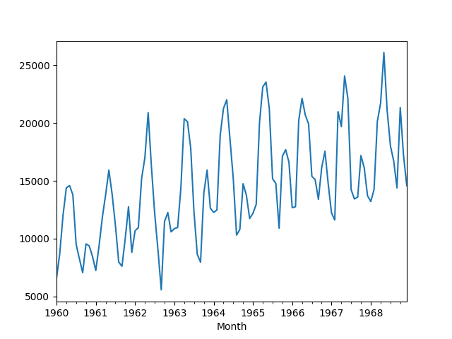
Monthly Car Sales Dataset Line Plot
Experimental Test Setup
It is important to evaluate time series forecasting models consistently.
In this section, we will define how we will evaluate the three forecast models in this tutorial.
First, we will hold the last two years of data back and evaluate forecasts on this data. Given the data is monthly, this means that the last 24 observations will be used as test data.
We will use a walk-forward validation method to evaluate model performance. This means that each time step in the test dataset will be enumerated, a model constructed on history data, and the forecast compared to the expected value. The observation will then be added to the training dataset and the process repeated.
Walk-forward validation is a realistic way to evaluate time series forecast models as one would expect models to be updated as new observations are made available.
Finally, forecasts will be evaluated using root mean squared error or RMSE. The benefit of RMSE is that it penalizes large errors and the scores are in the same units as the forecast values (car sales per month).
In summary, the test harness involves:
- The last 2 years of data used a test set.
- Walk-forward validation for model evaluation.
- Root mean squared error used to report model skill.
Optimized Persistence Forecast
The persistence forecast involves using the previous observation to predict the next time step.
For this reason, the approach is often called the naive forecast.
Why stop with using the previous observation? In this section, we will look at automating the persistence forecast and evaluate the use of any arbitrary prior time step to predict the next time step.
We will explore using each of the prior 24 months of point observations in a persistence model. Each configuration will be evaluated using the test harness and RMSE scores collected. We will then display the scores and graph the relationship between the persisted time step and the model skill.
The complete example is listed below.
|
1 2 3 4 5 6 7 8 9 10 11 12 13 14 15 16 17 18 19 20 21 22 23 24 25 26 27 28 |
from pandas import read_csv from sklearn.metrics import mean_squared_error from math import sqrt from matplotlib import pyplot # load data series = read_csv('car-sales.csv', header=0, index_col=0) # prepare data X = series.values train, test = X[0:-24], X[-24:] persistence_values = range(1, 25) scores = list() for p in persistence_values: # walk-forward validation history = [x for x in train] predictions = list() for i in range(len(test)): # make prediction yhat = history[-p] predictions.append(yhat) # observation history.append(test[i]) # report performance rmse = sqrt(mean_squared_error(test, predictions)) scores.append(rmse) print('p=%d RMSE:%.3f' % (p, rmse)) # plot scores over persistence values pyplot.plot(persistence_values, scores) pyplot.show() |
Running the example prints the RMSE for each persisted point observation.
|
1 2 3 4 5 6 7 8 9 10 11 12 13 14 15 16 17 18 19 20 21 22 23 24 |
p=1 RMSE:3947.200 p=2 RMSE:5485.353 p=3 RMSE:6346.176 p=4 RMSE:6474.553 p=5 RMSE:5756.543 p=6 RMSE:5756.076 p=7 RMSE:5958.665 p=8 RMSE:6543.266 p=9 RMSE:6450.839 p=10 RMSE:5595.971 p=11 RMSE:3806.482 p=12 RMSE:1997.732 p=13 RMSE:3968.987 p=14 RMSE:5210.866 p=15 RMSE:6299.040 p=16 RMSE:6144.881 p=17 RMSE:5349.691 p=18 RMSE:5534.784 p=19 RMSE:5655.016 p=20 RMSE:6746.872 p=21 RMSE:6784.611 p=22 RMSE:5642.737 p=23 RMSE:3692.062 p=24 RMSE:2119.103 |
A plot of the persisted value (t-n) to model skill (RMSE) is also created.
From the results, it is clear that persisting the observation from 12 months ago or 24 months ago is a great starting point on this dataset.
The best result achieved involved persisting the result from t-12 with an RMSE of 1997.732 car sales.
This is an obvious result, but also very useful.
We would expect that a forecast model that is some weighted combination of the observations at t-12, t-24, t-36 and so on would be a powerful starting point.
It also points out that the naive t-1 persistence would have been a less desirable starting point on this dataset.
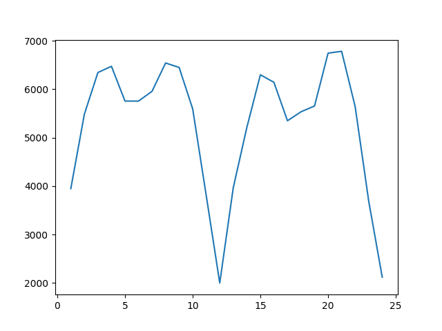
Persisted Observation to RMSE on the Monthly Car Sales Dataset
We can use the t-12 model to make a prediction and plot it against the test data.
The complete example is listed below.
|
1 2 3 4 5 6 7 8 9 10 11 12 13 14 15 16 17 18 19 20 21 22 |
from pandas import read_csv from sklearn.metrics import mean_squared_error from math import sqrt from matplotlib import pyplot # load data series = read_csv('car-sales.csv', header=0, index_col=0) # prepare data X = series.values train, test = X[0:-24], X[-24:] # walk-forward validation history = [x for x in train] predictions = list() for i in range(len(test)): # make prediction yhat = history[-12] predictions.append(yhat) # observation history.append(test[i]) # plot predictions vs observations pyplot.plot(test) pyplot.plot(predictions) pyplot.show() |
Running the example plots the test dataset (blue) against the predicted values (orange).
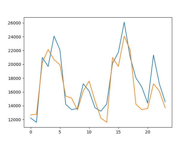
Line Plot of Predicted Values vs Test Dataset for the t-12 Persistence Model
You can learn more about the persistence model for time series forecasting in the post:
Expanding Window Forecast
An expanding window refers to a model that calculates a statistic on all available historic data and uses that to make a forecast.
It is an expanding window because it grows as more real observations are collected.
Two good starting point statistics to calculate are the mean and the median historical observation.
The example below uses the expanding window mean as the forecast.
|
1 2 3 4 5 6 7 8 9 10 11 12 13 14 15 16 17 18 19 20 21 |
from pandas import read_csv from sklearn.metrics import mean_squared_error from math import sqrt from numpy import mean # load data series = read_csv('car-sales.csv', header=0, index_col=0) # prepare data X = series.values train, test = X[0:-24], X[-24:] # walk-forward validation history = [x for x in train] predictions = list() for i in range(len(test)): # make prediction yhat = mean(history) predictions.append(yhat) # observation history.append(test[i]) # report performance rmse = sqrt(mean_squared_error(test, predictions)) print('RMSE: %.3f' % rmse) |
Running the example prints the RMSE evaluation of the approach.
|
1 |
RMSE: 5113.067 |
We can also repeat the same experiment with the median of the historical observations. The complete example is listed below.
|
1 2 3 4 5 6 7 8 9 10 11 12 13 14 15 16 17 18 19 20 21 |
from pandas import read_csv from sklearn.metrics import mean_squared_error from math import sqrt from numpy import median # load data series = read_csv('car-sales.csv', header=0, index_col=0) # prepare data X = series.values train, test = X[0:-24], X[-24:] # walk-forward validation history = [x for x in train] predictions = list() for i in range(len(test)): # make prediction yhat = median(history) predictions.append(yhat) # observation history.append(test[i]) # report performance rmse = sqrt(mean_squared_error(test, predictions)) print('RMSE: %.3f' % rmse) |
Again, running the example prints the skill of the model.
We can see that on this problem the historical mean produced a better result than the median, but both were worse models than using the optimized persistence values.
|
1 |
RMSE: 5527.408 |
We can plot the mean expanding window predictions against the test dataset to get a feeling for how the forecast actually looks in context.
The complete example is listed below.
|
1 2 3 4 5 6 7 8 9 10 11 12 13 14 15 16 17 18 19 20 21 22 |
from pandas import read_csv from sklearn.metrics import mean_squared_error from matplotlib import pyplot from numpy import mean # load data series = read_csv('car-sales.csv', header=0, index_col=0) # prepare data X = series.values train, test = X[0:-24], X[-24:] # walk-forward validation history = [x for x in train] predictions = list() for i in range(len(test)): # make prediction yhat = mean(history) predictions.append(yhat) # observation history.append(test[i]) # plot predictions vs observations pyplot.plot(test) pyplot.plot(predictions) pyplot.show() |
The plot shows what a poor forecast looks like and how it does not follow the movements of the data at all, other than a slight rising trend.
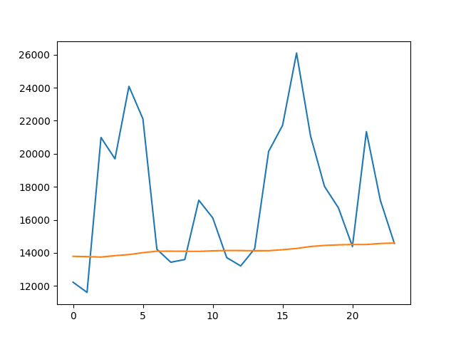
Line Plot of Predicted Values vs Test Dataset for the Mean Expanding Window Model
You can see more examples of expanding window statistics in the post:
Rolling Window Forecast
A rolling window model involves calculating a statistic on a fixed contiguous block of prior observations and using it as a forecast.
It is much like the expanding window, but the window size remains fixed and counts backwards from the most recent observation.
It may be more useful on time series problems where recent lag values are more predictive than older lag values.
We will automatically check different rolling window sizes from 1 to 24 months (2 years) and start by calculating the mean observation and using that as a forecast. The complete example is listed below.
|
1 2 3 4 5 6 7 8 9 10 11 12 13 14 15 16 17 18 19 20 21 22 23 24 25 26 27 28 29 |
from pandas import read_csv from sklearn.metrics import mean_squared_error from math import sqrt from matplotlib import pyplot from numpy import mean # load data series = read_csv('car-sales.csv', header=0, index_col=0) # prepare data X = series.values train, test = X[0:-24], X[-24:] window_sizes = range(1, 25) scores = list() for w in window_sizes: # walk-forward validation history = [x for x in train] predictions = list() for i in range(len(test)): # make prediction yhat = mean(history[-w:]) predictions.append(yhat) # observation history.append(test[i]) # report performance rmse = sqrt(mean_squared_error(test, predictions)) scores.append(rmse) print('w=%d RMSE:%.3f' % (w, rmse)) # plot scores over window sizes values pyplot.plot(window_sizes, scores) pyplot.show() |
Running the example prints the rolling window size and RMSE for each configuration.
|
1 2 3 4 5 6 7 8 9 10 11 12 13 14 15 16 17 18 19 20 21 22 23 24 |
w=1 RMSE:3947.200 w=2 RMSE:4350.413 w=3 RMSE:4701.446 w=4 RMSE:4810.510 w=5 RMSE:4649.667 w=6 RMSE:4549.172 w=7 RMSE:4515.684 w=8 RMSE:4614.551 w=9 RMSE:4653.493 w=10 RMSE:4563.802 w=11 RMSE:4321.599 w=12 RMSE:4023.968 w=13 RMSE:3901.634 w=14 RMSE:3907.671 w=15 RMSE:4017.276 w=16 RMSE:4084.080 w=17 RMSE:4076.399 w=18 RMSE:4085.376 w=19 RMSE:4101.505 w=20 RMSE:4195.617 w=21 RMSE:4269.784 w=22 RMSE:4258.226 w=23 RMSE:4158.029 w=24 RMSE:4021.885 |
A line plot of window size to error is also created.
The results suggest that a rolling window of w=13 was best with an RMSE of 3,901 monthly car sales.
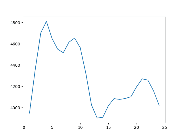
Line Plot of Rolling Window Size to RMSE for a Mean Forecast on the Monthly Car Sales Dataset
We can repeat this experiment with the median statistic.
The complete example is listed below.
|
1 2 3 4 5 6 7 8 9 10 11 12 13 14 15 16 17 18 19 20 21 22 23 24 25 26 27 28 29 |
from pandas import read_csv from sklearn.metrics import mean_squared_error from math import sqrt from matplotlib import pyplot from numpy import median # load data series = read_csv('car-sales.csv', header=0, index_col=0) # prepare data X = series.values train, test = X[0:-24], X[-24:] window_sizes = range(1, 25) scores = list() for w in window_sizes: # walk-forward validation history = [x for x in train] predictions = list() for i in range(len(test)): # make prediction yhat = median(history[-w:]) predictions.append(yhat) # observation history.append(test[i]) # report performance rmse = sqrt(mean_squared_error(test, predictions)) scores.append(rmse) print('w=%d RMSE:%.3f' % (w, rmse)) # plot scores over window sizes values pyplot.plot(window_sizes, scores) pyplot.show() |
Running the example again prints the window size and RMSE for each configuration.
|
1 2 3 4 5 6 7 8 9 10 11 12 13 14 15 16 17 18 19 20 21 22 23 24 |
w=1 RMSE:3947.200 w=2 RMSE:4350.413 w=3 RMSE:4818.406 w=4 RMSE:4993.473 w=5 RMSE:5212.887 w=6 RMSE:5002.830 w=7 RMSE:4958.621 w=8 RMSE:4817.664 w=9 RMSE:4932.317 w=10 RMSE:4928.661 w=11 RMSE:4885.574 w=12 RMSE:4414.139 w=13 RMSE:4204.665 w=14 RMSE:4172.579 w=15 RMSE:4382.037 w=16 RMSE:4522.304 w=17 RMSE:4494.803 w=18 RMSE:4360.445 w=19 RMSE:4232.285 w=20 RMSE:4346.389 w=21 RMSE:4465.536 w=22 RMSE:4514.596 w=23 RMSE:4428.739 w=24 RMSE:4236.126 |
A plot of the window size and RMSE is again created.
Here, we can see that best results were achieved with a window size of w=1 with an RMSE of 3947.200 monthly car sales, which was essentially a t-1 persistence model.
The results were generally worse than optimized persistence, but better than the expanding window model. We could imagine better results with a weighted combination of window observations, this idea leads to using linear models such as AR and ARIMA.
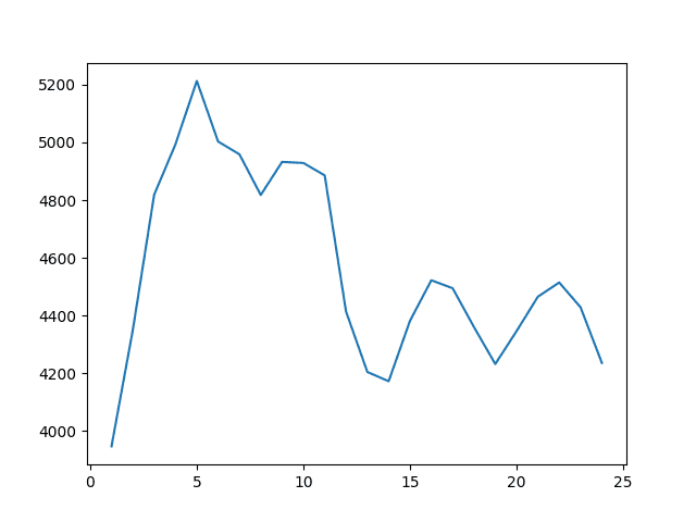
Line Plot of Rolling Window Size to RMSE for a Median Forecast on the Monthly Car Sales Dataset
Again, we can plot the predictions from the better model (mean rolling window with w=13) against the actual observations to get a feeling for how the forecast looks in context.
The complete example is listed below.
|
1 2 3 4 5 6 7 8 9 10 11 12 13 14 15 16 17 18 19 20 21 22 |
from pandas import read_csv from sklearn.metrics import mean_squared_error from matplotlib import pyplot from numpy import mean # load data series = read_csv('car-sales.csv', header=0, index_col=0) # prepare data X = series.values train, test = X[0:-24], X[-24:] # walk-forward validation history = [x for x in train] predictions = list() for i in range(len(test)): # make prediction yhat = mean(history[-13:]) predictions.append(yhat) # observation history.append(test[i]) # plot predictions vs observations pyplot.plot(test) pyplot.plot(predictions) pyplot.show() |
Running the code creates the line plot of observations (blue) compared to the predicted values (orange).
We can see that the model better follows the level of the data, but again does not follow the actual up and down movements.
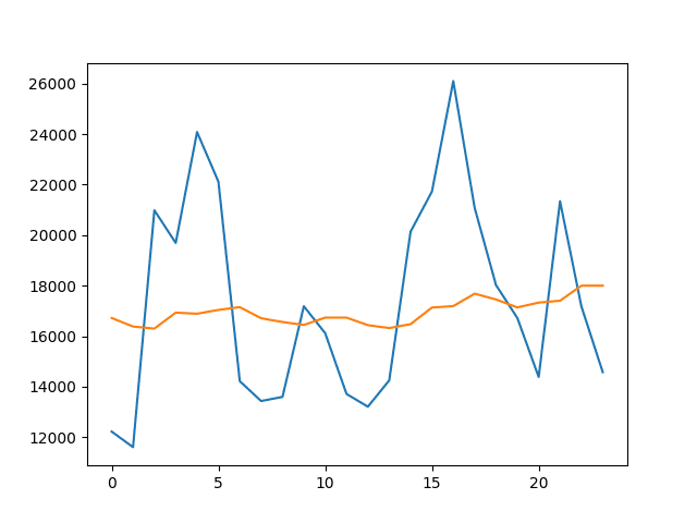
Line Plot of Predicted Values vs Test Dataset for the Mean w=13 Rolling Window Model
You can see more examples of rolling window statistics in the post:
Summary
In this tutorial, you discovered the importance of calculating the worst acceptable performance on a time series forecasting problem and methods that you can use to ensure you are not fooling yourself with more sophisticated methods.
Specifically, you learned:
- How to automatically test a suite of persistence configurations.
- How to evaluate an expanding window model.
- How to automatically test a suite of rolling window configurations.
Do you have any questions about baseline forecasting methods, or about this post?
Ask your questions in the comments and I will do my best to answer.
Want to Develop Time Series Forecasts with Python?

Develop Your Own Forecasts in Minutes
...with just a few lines of python codeDiscover how in my new Ebook:
Introduction to Time Series Forecasting With Python
It covers self-study tutorials and end-to-end projects on topics like: Loading data, visualization, modeling, algorithm tuning, and much more...
Finally Bring Time Series Forecasting to
Your Own Projects
Skip the Academics. Just Results.


zero comments? for such an informative, well-written and essential post? a travesty.
Thanks.
What’s the right way to select the testing split size? All I’ve found is that typically you choose 20% of the data, as a general formula.
There is no best way. The test set must be representative.
Perhaps try different sizes and compare results.
Perhaps talk to domain experts for your data.
used these methods for my thesis research. Thanks for this beautiful post.
Well done!
Hi! This is such a great post!
I’m having a bit of trouble understanding Python codes, though. In the first Python codes under the Optimized Persistence Forecast how is yhat computed?
Is it the mean of the past values of p (persistence values)?
Thank you so much
No, it just finds the best negative offset (-1, -2, -3, …) to use for a persistence model.
Do these models predict future time steps beyond the data set? Or are they predicting the window of the held back data?
You can use them any way you like.
We always evaluate models based on the skill of their predictions on data not seen during training.
I did not understand why we are adding the test data(test[i]) to historical data while predicting.
That is to compare with prediction to see how good are we doing.
Hi there,
Thank you for the insightful post. I am working with an imbalanced dataset (target is only shown in 15% of the total months). I need to fix this imbalance. However, should I do this on the training set before the cross-validation, or can I somehow implement an imbalance fix into the rolling window code so that an imbalance fixer is done within each window? I am unsure on what is best both theoretically and practically here, so any insight would be much appreciated!
Hi JK…The following resource may be of interest to you:
https://arxiv.org/abs/2107.10709
Hi James, thank you for your response – that is a very helpful paper, I’ll be sure to incorporate it into my research. However, my current project is framed as a classification problem (apologies for not mentioning this before!) despite being time series. As per this article: https://machinelearningmastery.com/smote-oversampling-for-imbalanced-classification/ I now believe that I must fix the imbalance within each CV window (in the same way that you must fix imbalance within each fold), not prior to running any CV. Would this be correct? If so, I am unsure how to incorporate imbalance fixing techniques into the rolling window CV generator effectively. Would this be somewhat easy to implement in Python? Unfortunately, I cannot find any examples online.
Thank you for your time 🙂