Deep learning neural networks are capable of automatically learning and extracting features from raw data.
This feature of neural networks can be used for time series forecasting problems, where models can be developed directly on the raw observations without the direct need to scale the data using normalization and standardization or to make the data stationary by differencing.
Impressively, simple deep learning neural network models are capable of making skillful forecasts as compared to naive models and tuned SARIMA models on univariate time series forecasting problems that have both trend and seasonal components with no pre-processing.
In this tutorial, you will discover how to develop a suite of deep learning models for univariate time series forecasting.
After completing this tutorial, you will know:
- How to develop a robust test harness using walk-forward validation for evaluating the performance of neural network models.
- How to develop and evaluate simple multilayer Perceptron and convolutional neural networks for time series forecasting.
- How to develop and evaluate LSTMs, CNN-LSTMs, and ConvLSTM neural network models for time series forecasting.
Kick-start your project with my new book Deep Learning for Time Series Forecasting, including step-by-step tutorials and the Python source code files for all examples.
Let’s get started.
- Updated Apr/2019: Updated the link to dataset.

How to Develop Deep Learning Models for Univariate Time Series Forecasting
Photo by Nathaniel McQueen, some rights reserved.
Tutorial Overview
This tutorial is divided into five parts; they are:
- Problem Description
- Model Evaluation Test Harness
- Multilayer Perceptron Model
- Convolutional Neural Network Model
- Recurrent Neural Network Models
Problem Description
The ‘monthly car sales‘ dataset summarizes the monthly car sales in Quebec, Canada between 1960 and 1968.
Download the dataset directly from here:
Save the file with the filename ‘monthly-car-sales.csv‘ in your current working directory.
We can load this dataset as a Pandas series using the function read_csv().
|
1 2 |
# load series = read_csv('monthly-car-sales.csv', header=0, index_col=0) |
Once loaded, we can summarize the shape of the dataset in order to determine the number of observations.
|
1 2 |
# summarize shape print(series.shape) |
We can then create a line plot of the series to get an idea of the structure of the series.
|
1 2 3 |
# plot pyplot.plot(series) pyplot.show() |
We can tie all of this together; the complete example is listed below.
|
1 2 3 4 5 6 7 8 9 10 |
# load and plot dataset from pandas import read_csv from matplotlib import pyplot # load series = read_csv('monthly-car-sales.csv', header=0, index_col=0) # summarize shape print(series.shape) # plot pyplot.plot(series) pyplot.show() |
Running the example first prints the shape of the dataset.
|
1 |
(108, 1) |
The dataset is monthly and has nine years, or 108 observations. In our testing, will use the last year, or 12 observations, as the test set.
A line plot is created. The dataset has an obvious trend and seasonal component. The period of the seasonal component could be six months or 12 months.
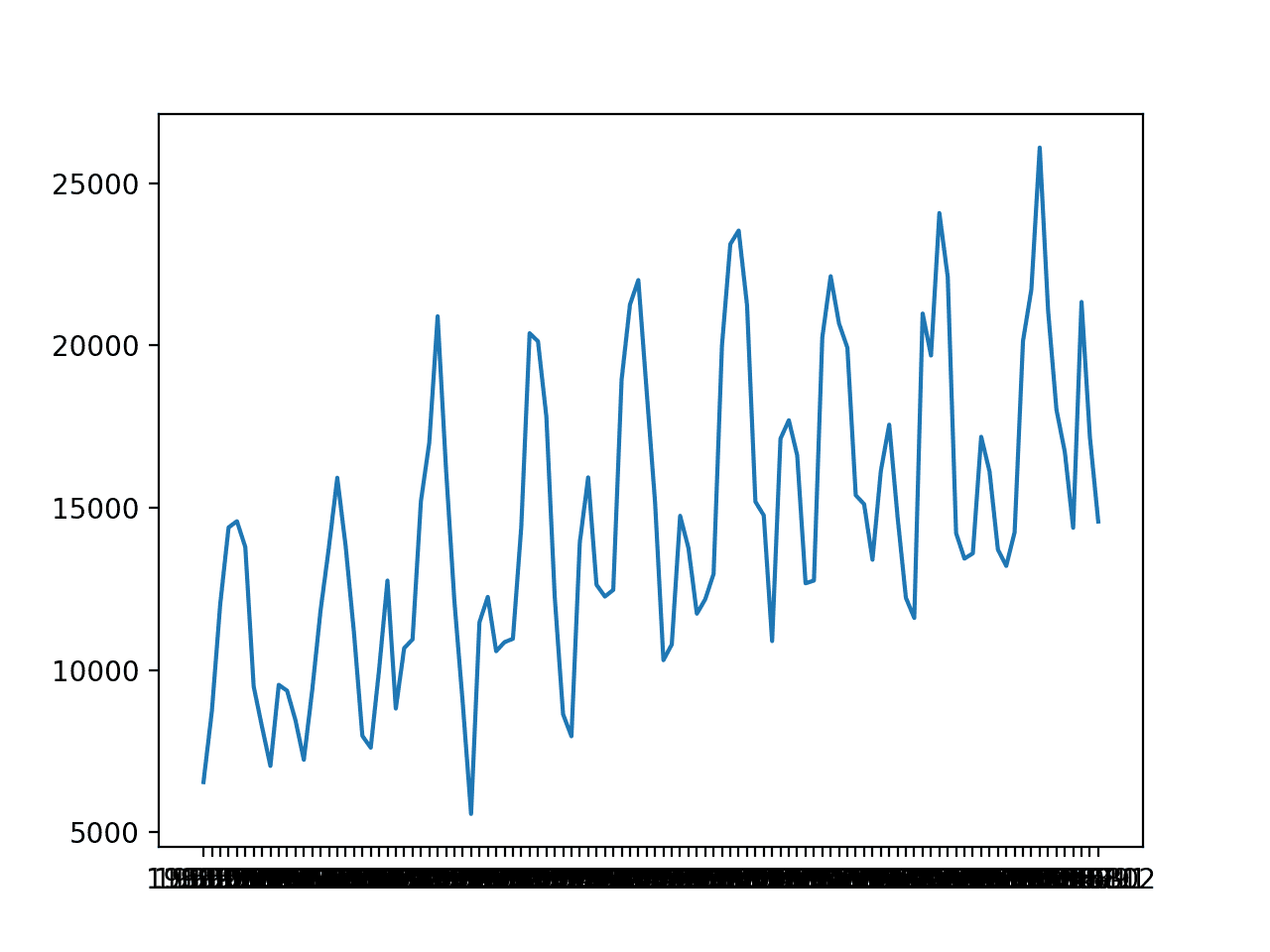
Line Plot of Monthly Car Sales
From prior experiments, we know that a naive model can achieve a root mean squared error, or RMSE, of 1841.155 by taking the median of the observations at the three prior years for the month being predicted; for example:
|
1 |
yhat = median(-12, -24, -36) |
Where the negative indexes refer to observations in the series relative to the end of the historical data for the month being predicted.
From prior experiments, we know that a SARIMA model can achieve an RMSE of 1551.842 with the configuration of SARIMA(0, 0, 0),(1, 1, 0),12 where no elements are specified for the trend and a seasonal difference with a period of 12 is calculated and an AR model of one season is used.
The performance of the naive model provides a lower bound on a model that is considered skillful. Any model that achieves a predictive performance of lower than 1841.155 on the last 12 months has skill.
The performance of the SARIMA model provides a measure of a good model on the problem. Any model that achieves a predictive performance lower than 1551.842 on the last 12 months should be adopted over a SARIMA model.
Now that we have defined our problem and expectations of model skill, we can look at defining the test harness.
Need help with Deep Learning for Time Series?
Take my free 7-day email crash course now (with sample code).
Click to sign-up and also get a free PDF Ebook version of the course.
Model Evaluation Test Harness
In this section, we will develop a test harness for developing and evaluating different types of neural network models for univariate time series forecasting.
This section is divided into the following parts:
- Train-Test Split
- Series as Supervised Learning
- Walk-Forward Validation
- Repeat Evaluation
- Summarize Performance
- Worked Example
Train-Test Split
The first step is to split the loaded series into train and test sets.
We will use the first eight years (96 observations) for training and the last 12 for the test set.
The train_test_split() function below will split the series taking the raw observations and the number of observations to use in the test set as arguments.
|
1 2 3 |
# split a univariate dataset into train/test sets def train_test_split(data, n_test): return data[:-n_test], data[-n_test:] |
Series as Supervised Learning
Next, we need to be able to frame the univariate series of observations as a supervised learning problem so that we can train neural network models.
A supervised learning framing of a series means that the data needs to be split into multiple examples that the model learn from and generalize across.
Each sample must have both an input component and an output component.
The input component will be some number of prior observations, such as three years or 36 time steps.
The output component will be the total sales in the next month because we are interested in developing a model to make one-step forecasts.
We can implement this using the shift() function on the pandas DataFrame. It allows us to shift a column down (forward in time) or back (backward in time). We can take the series as a column of data, then create multiple copies of the column, shifted forward or backward in time in order to create the samples with the input and output elements we require.
When a series is shifted down, NaN values are introduced because we don’t have values beyond the start of the series.
For example, the series defined as a column:
|
1 2 3 4 5 |
(t) 1 2 3 4 |
Can be shifted and inserted as a column beforehand:
|
1 2 3 4 5 6 |
(t-1), (t) Nan, 1 1, 2 2, 3 3, 4 4 NaN |
We can see that on the second row, the value 1 is provided as input as an observation at the prior time step, and 2 is the next value in the series that can be predicted, or learned by the model to be predicted when 1 is presented as input.
Rows with NaN values can be removed.
The series_to_supervised() function below implements this behavior, allowing you to specify the number of lag observations to use in the input and the number to use in the output for each sample. It will also remove rows that have NaN values as they cannot be used to train or test a model.
|
1 2 3 4 5 6 7 8 9 10 11 12 13 14 15 |
# transform list into supervised learning format def series_to_supervised(data, n_in=1, n_out=1): df = DataFrame(data) cols = list() # input sequence (t-n, ... t-1) for i in range(n_in, 0, -1): cols.append(df.shift(i)) # forecast sequence (t, t+1, ... t+n) for i in range(0, n_out): cols.append(df.shift(-i)) # put it all together agg = concat(cols, axis=1) # drop rows with NaN values agg.dropna(inplace=True) return agg.values |
Walk-Forward Validation
Time series forecasting models can be evaluated on a test set using walk-forward validation.
Walk-forward validation is an approach where the model makes a forecast for each observation in the test dataset one at a time. After each forecast is made for a time step in the test dataset, the true observation for the forecast is added to the test dataset and made available to the model.
Simpler models can be refit with the observation prior to making the subsequent prediction. More complex models, such as neural networks, are not refit given the much greater computational cost.
Nevertheless, the true observation for the time step can then be used as part of the input for making the prediction on the next time step.
First, the dataset is split into train and test sets. We will call the train_test_split() function to perform this split and pass in the pre-specified number of observations to use as the test data.
A model will be fit once on the training dataset for a given configuration.
We will define a generic model_fit() function to perform this operation that can be filled in for the given type of neural network that we may be interested in later. The function takes the training dataset and the model configuration and returns the fit model ready for making predictions.
|
1 2 3 |
# fit a model def model_fit(train, config): return None |
Each time step of the test dataset is enumerated. A prediction is made using the fit model.
Again, we will define a generic function named model_predict() that takes the fit model, the history, and the model configuration and makes a single one-step prediction.
|
1 2 3 |
# forecast with a pre-fit model def model_predict(model, history, config): return 0.0 |
The prediction is added to a list of predictions and the true observation from the test set is added to a list of observations that was seeded with all observations from the training dataset. This list is built up during each step in the walk-forward validation, allowing the model to make a one-step prediction using the most recent history.
All of the predictions can then be compared to the true values in the test set and an error measure calculated.
We will calculate the root mean squared error, or RMSE, between predictions and the true values.
RMSE is calculated as the square root of the average of the squared differences between the forecasts and the actual values. The measure_rmse() implements this below using the mean_squared_error() scikit-learn function to first calculate the mean squared error, or MSE, before calculating the square root.
|
1 2 3 |
# root mean squared error or rmse def measure_rmse(actual, predicted): return sqrt(mean_squared_error(actual, predicted)) |
The complete walk_forward_validation() function that ties all of this together is listed below.
It takes the dataset, the number of observations to use as the test set, and the configuration for the model, and returns the RMSE for the model performance on the test set.
|
1 2 3 4 5 6 7 8 9 10 11 12 13 14 15 16 17 18 19 20 21 |
# walk-forward validation for univariate data def walk_forward_validation(data, n_test, cfg): predictions = list() # split dataset train, test = train_test_split(data, n_test) # fit model model = model_fit(train, cfg) # seed history with training dataset history = [x for x in train] # step over each time-step in the test set for i in range(len(test)): # fit model and make forecast for history yhat = model_predict(model, history, cfg) # store forecast in list of predictions predictions.append(yhat) # add actual observation to history for the next loop history.append(test[i]) # estimate prediction error error = measure_rmse(test, predictions) print(' > %.3f' % error) return error |
Repeat Evaluation
Neural network models are stochastic.
This means that, given the same model configuration and the same training dataset, a different internal set of weights will result each time the model is trained that will in turn have a different performance.
This is a benefit, allowing the model to be adaptive and find high performing configurations to complex problems.
It is also a problem when evaluating the performance of a model and in choosing a final model to use to make predictions.
To address model evaluation, we will evaluate a model configuration multiple times via walk-forward validation and report the error as the average error across each evaluation.
This is not always possible for large neural networks and may only make sense for small networks that can be fit in minutes or hours.
The repeat_evaluate() function below implements this and allows the number of repeats to be specified as an optional parameter that defaults to 30 and returns a list of model performance scores: in this case, RMSE values.
|
1 2 3 4 5 |
# repeat evaluation of a config def repeat_evaluate(data, config, n_test, n_repeats=30): # fit and evaluate the model n times scores = [walk_forward_validation(data, n_test, config) for _ in range(n_repeats)] return scores |
Summarize Performance
Finally, we need to summarize the performance of a model from the multiple repeats.
We will summarize the performance first using summary statistics, specifically the mean and the standard deviation.
We will also plot the distribution of model performance scores using a box and whisker plot to help get an idea of the spread of performance.
The summarize_scores() function below implements this, taking the name of the model that was evaluated and the list of scores from each repeated evaluation, printing the summary and showing a plot.
|
1 2 3 4 5 6 7 8 |
# summarize model performance def summarize_scores(name, scores): # print a summary scores_m, score_std = mean(scores), std(scores) print('%s: %.3f RMSE (+/- %.3f)' % (name, scores_m, score_std)) # box and whisker plot pyplot.boxplot(scores) pyplot.show() |
Worked Example
Now that we have defined the elements of the test harness, we can tie them all together and define a simple persistence model.
Specifically, we will calculate the median of a subset of prior observations relative to the time to be forecasted.
We do not need to fit a model so the model_fit() function will be implemented to simply return None.
|
1 2 3 |
# fit a model def model_fit(train, config): return None |
We will use the config to define a list of index offsets in the prior observations relative to the time to be forecasted that will be used as the prediction. For example, 12 will use the observation 12 months ago (-12) relative to the time to be forecasted.
|
1 2 |
# define config config = [12, 24, 36] |
The model_predict() function can be implemented to use this configuration to collect the observations, then return the median of those observations.
|
1 2 3 4 5 6 |
# forecast with a pre-fit model def model_predict(model, history, config): values = list() for offset in config: values.append(history[-offset]) return median(values) |
The complete example of using the framework with a simple persistence model is listed below.
|
1 2 3 4 5 6 7 8 9 10 11 12 13 14 15 16 17 18 19 20 21 22 23 24 25 26 27 28 29 30 31 32 33 34 35 36 37 38 39 40 41 42 43 44 45 46 47 48 49 50 51 52 53 54 55 56 57 58 59 60 61 62 63 64 65 66 67 68 69 70 71 72 73 74 75 76 77 78 79 80 81 82 83 84 85 86 87 88 89 90 91 92 93 94 95 96 |
# persistence from math import sqrt from numpy import mean from numpy import std from pandas import DataFrame from pandas import concat from pandas import read_csv from sklearn.metrics import mean_squared_error from matplotlib import pyplot # split a univariate dataset into train/test sets def train_test_split(data, n_test): return data[:-n_test], data[-n_test:] # transform list into supervised learning format def series_to_supervised(data, n_in=1, n_out=1): df = DataFrame(data) cols = list() # input sequence (t-n, ... t-1) for i in range(n_in, 0, -1): cols.append(df.shift(i)) # forecast sequence (t, t+1, ... t+n) for i in range(0, n_out): cols.append(df.shift(-i)) # put it all together agg = concat(cols, axis=1) # drop rows with NaN values agg.dropna(inplace=True) return agg.values # root mean squared error or rmse def measure_rmse(actual, predicted): return sqrt(mean_squared_error(actual, predicted)) # difference dataset def difference(data, interval): return [data[i] - data[i - interval] for i in range(interval, len(data))] # fit a model def model_fit(train, config): return None # forecast with a pre-fit model def model_predict(model, history, config): values = list() for offset in config: values.append(history[-offset]) return median(values) # walk-forward validation for univariate data def walk_forward_validation(data, n_test, cfg): predictions = list() # split dataset train, test = train_test_split(data, n_test) # fit model model = model_fit(train, cfg) # seed history with training dataset history = [x for x in train] # step over each time-step in the test set for i in range(len(test)): # fit model and make forecast for history yhat = model_predict(model, history, cfg) # store forecast in list of predictions predictions.append(yhat) # add actual observation to history for the next loop history.append(test[i]) # estimate prediction error error = measure_rmse(test, predictions) print(' > %.3f' % error) return error # repeat evaluation of a config def repeat_evaluate(data, config, n_test, n_repeats=30): # fit and evaluate the model n times scores = [walk_forward_validation(data, n_test, config) for _ in range(n_repeats)] return scores # summarize model performance def summarize_scores(name, scores): # print a summary scores_m, score_std = mean(scores), std(scores) print('%s: %.3f RMSE (+/- %.3f)' % (name, scores_m, score_std)) # box and whisker plot pyplot.boxplot(scores) pyplot.show() series = read_csv('monthly-car-sales.csv', header=0, index_col=0) data = series.values # data split n_test = 12 # define config config = [12, 24, 36] # grid search scores = repeat_evaluate(data, config, n_test) # summarize scores summarize_scores('persistence', scores) |
Running the example prints the RMSE of the model evaluated using walk-forward validation on the final 12 months of data.
The model is evaluated 30 times, although, because the model has no stochastic element, the score is the same each time.
|
1 2 3 4 5 6 7 8 9 10 11 12 13 14 15 16 17 18 19 20 21 22 23 24 25 26 27 28 29 30 31 |
> 1841.156 > 1841.156 > 1841.156 > 1841.156 > 1841.156 > 1841.156 > 1841.156 > 1841.156 > 1841.156 > 1841.156 > 1841.156 > 1841.156 > 1841.156 > 1841.156 > 1841.156 > 1841.156 > 1841.156 > 1841.156 > 1841.156 > 1841.156 > 1841.156 > 1841.156 > 1841.156 > 1841.156 > 1841.156 > 1841.156 > 1841.156 > 1841.156 > 1841.156 > 1841.156 persistence: 1841.156 RMSE (+/- 0.000) |
We can see that the RMSE of the model is 1841, providing a lower-bound of performance by which we can evaluate whether a model is skillful or not on the problem.
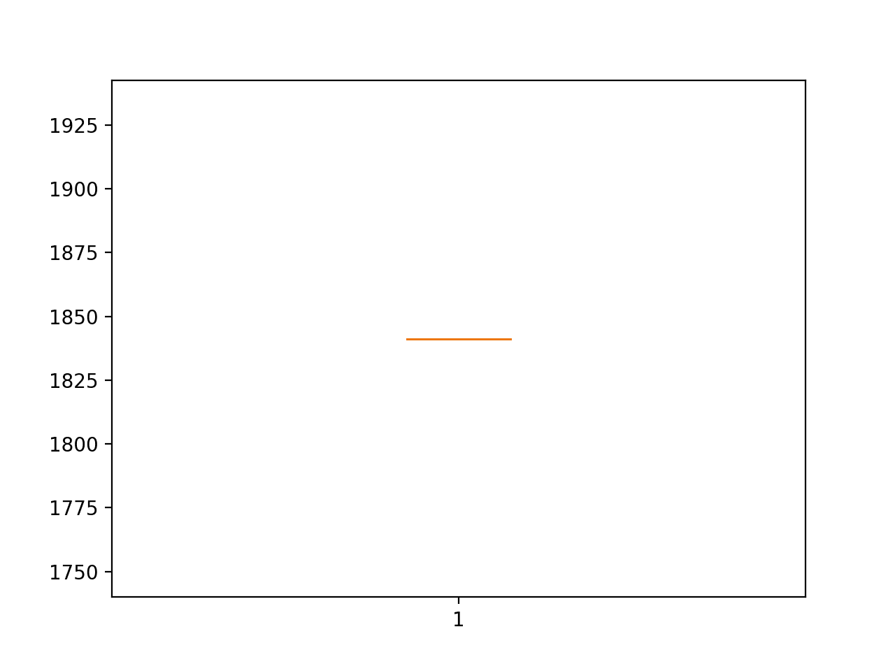
Box and Whisker Plot of Persistence RMSE Forecasting Car Sales
Now that we have a robust test harness, we can use it to evaluate a suite of neural network models.
Multilayer Perceptron Model
The first network that we will evaluate is a multilayer Perceptron, or MLP for short.
This is a simple feed-forward neural network model that should be evaluated before more elaborate models are considered.
MLPs can be used for time series forecasting by taking multiple observations at prior time steps, called lag observations, and using them as input features and predicting one or more time steps from those observations.
This is exactly the framing of the problem provided by the series_to_supervised() function in the previous section.
The training dataset is therefore a list of samples, where each sample has some number of observations from months prior to the time being forecasted, and the forecast is the next month in the sequence. For example:
|
1 2 3 4 5 |
X, y month1, month2, month3, month4 month2, month3, month4, month5 month3, month4, month5, month6 ... |
The model will attempt to generalize over these samples, such that when a new sample is provided beyond what is known by the model, it can predict something useful; for example:
|
1 2 |
X, y month4, month5, month6, ??? |
We will implement a simple MLP using the Keras deep learning library.
The model will have an input layer with some number of prior observations. This can be specified using the input_dim argument when we define the first hidden layer. The model will have a single hidden layer with some number of nodes, then a single output layer.
We will use the rectified linear activation function on the hidden layer as it performs well. We will use a linear activation function (the default) on the output layer because we are predicting a continuous value.
The loss function for the network will be the mean squared error loss, or MSE, and we will use the efficient Adam flavor of stochastic gradient descent to train the network.
|
1 2 3 4 5 |
# define model model = Sequential() model.add(Dense(n_nodes, activation='relu', input_dim=n_input)) model.add(Dense(1)) model.compile(loss='mse', optimizer='adam') |
The model will be fit for some number of training epochs (exposures to the training data) and batch size can be specified to define how often the weights are updated within each epoch.
The model_fit() function for fitting an MLP model on the training dataset is listed below.
The function expects the config to be a list with the following configuration hyperparameters:
- n_input: The number of lag observations to use as input to the model.
- n_nodes: The number of nodes to use in the hidden layer.
- n_epochs: The number of times to expose the model to the whole training dataset.
- n_batch: The number of samples within an epoch after which the weights are updated.
|
1 2 3 4 5 6 7 8 9 10 11 12 13 14 15 |
# fit a model def model_fit(train, config): # unpack config n_input, n_nodes, n_epochs, n_batch = config # prepare data data = series_to_supervised(train, n_in=n_input) train_x, train_y = data[:, :-1], data[:, -1] # define model model = Sequential() model.add(Dense(n_nodes, activation='relu', input_dim=n_input)) model.add(Dense(1)) model.compile(loss='mse', optimizer='adam') # fit model.fit(train_x, train_y, epochs=n_epochs, batch_size=n_batch, verbose=0) return model |
Making a prediction with a fit MLP model is as straightforward as calling the predict() function and passing in one sample worth of input values required to make the prediction.
|
1 |
yhat = model.predict(x_input, verbose=0) |
In order to make a prediction beyond the limit of known data, this requires that the last n known observations are taken as an array and used as input.
The predict() function expects one or more samples of inputs when making a prediction, so providing a single sample requires the array to have the shape [1, n_input], where n_input is the number of time steps that the model expects as input.
Similarly, the predict() function returns an array of predictions, one for each sample provided as input. In the case of one prediction, there will be an array with one value.
The model_predict() function below implements this behavior, taking the model, the prior observations, and model configuration as arguments, formulating an input sample and making a one-step prediction that is then returned.
|
1 2 3 4 5 6 7 8 9 |
# forecast with a pre-fit model def model_predict(model, history, config): # unpack config n_input, _, _, _ = config # prepare data x_input = array(history[-n_input:]).reshape(1, n_input) # forecast yhat = model.predict(x_input, verbose=0) return yhat[0] |
We now have everything we need to evaluate an MLP model on the monthly car sales dataset.
A simple grid search of model hyperparameters was performed and the configuration below was chosen. This may not be an optimal configuration, but is the best that was found.
- n_input: 24 (e.g. 24 months)
- n_nodes: 500
- n_epochs: 100
- n_batch: 100
This configuration can be defined as a list:
|
1 2 |
# define config config = [24, 500, 100, 100] |
Note that when the training data is framed as a supervised learning problem, there are only 72 samples that can be used to train the model.
Using a batch size of 72 or more means that the model is being trained using batch gradient descent instead of mini-batch gradient descent. This is often used for small datasets and means that weight updates and gradient calculations are performed at the end of each epoch, instead of multiple times within each epoch.
The complete code example is listed below.
|
1 2 3 4 5 6 7 8 9 10 11 12 13 14 15 16 17 18 19 20 21 22 23 24 25 26 27 28 29 30 31 32 33 34 35 36 37 38 39 40 41 42 43 44 45 46 47 48 49 50 51 52 53 54 55 56 57 58 59 60 61 62 63 64 65 66 67 68 69 70 71 72 73 74 75 76 77 78 79 80 81 82 83 84 85 86 87 88 89 90 91 92 93 94 95 96 97 98 99 100 101 102 103 104 105 106 107 108 109 110 |
# evaluate mlp from math import sqrt from numpy import array from numpy import mean from numpy import std from pandas import DataFrame from pandas import concat from pandas import read_csv from sklearn.metrics import mean_squared_error from keras.models import Sequential from keras.layers import Dense from matplotlib import pyplot # split a univariate dataset into train/test sets def train_test_split(data, n_test): return data[:-n_test], data[-n_test:] # transform list into supervised learning format def series_to_supervised(data, n_in=1, n_out=1): df = DataFrame(data) cols = list() # input sequence (t-n, ... t-1) for i in range(n_in, 0, -1): cols.append(df.shift(i)) # forecast sequence (t, t+1, ... t+n) for i in range(0, n_out): cols.append(df.shift(-i)) # put it all together agg = concat(cols, axis=1) # drop rows with NaN values agg.dropna(inplace=True) return agg.values # root mean squared error or rmse def measure_rmse(actual, predicted): return sqrt(mean_squared_error(actual, predicted)) # fit a model def model_fit(train, config): # unpack config n_input, n_nodes, n_epochs, n_batch = config # prepare data data = series_to_supervised(train, n_in=n_input) train_x, train_y = data[:, :-1], data[:, -1] # define model model = Sequential() model.add(Dense(n_nodes, activation='relu', input_dim=n_input)) model.add(Dense(1)) model.compile(loss='mse', optimizer='adam') # fit model.fit(train_x, train_y, epochs=n_epochs, batch_size=n_batch, verbose=0) return model # forecast with a pre-fit model def model_predict(model, history, config): # unpack config n_input, _, _, _ = config # prepare data x_input = array(history[-n_input:]).reshape(1, n_input) # forecast yhat = model.predict(x_input, verbose=0) return yhat[0] # walk-forward validation for univariate data def walk_forward_validation(data, n_test, cfg): predictions = list() # split dataset train, test = train_test_split(data, n_test) # fit model model = model_fit(train, cfg) # seed history with training dataset history = [x for x in train] # step over each time-step in the test set for i in range(len(test)): # fit model and make forecast for history yhat = model_predict(model, history, cfg) # store forecast in list of predictions predictions.append(yhat) # add actual observation to history for the next loop history.append(test[i]) # estimate prediction error error = measure_rmse(test, predictions) print(' > %.3f' % error) return error # repeat evaluation of a config def repeat_evaluate(data, config, n_test, n_repeats=30): # fit and evaluate the model n times scores = [walk_forward_validation(data, n_test, config) for _ in range(n_repeats)] return scores # summarize model performance def summarize_scores(name, scores): # print a summary scores_m, score_std = mean(scores), std(scores) print('%s: %.3f RMSE (+/- %.3f)' % (name, scores_m, score_std)) # box and whisker plot pyplot.boxplot(scores) pyplot.show() series = read_csv('monthly-car-sales.csv', header=0, index_col=0) data = series.values # data split n_test = 12 # define config config = [24, 500, 100, 100] # grid search scores = repeat_evaluate(data, config, n_test) # summarize scores summarize_scores('mlp', scores) |
Running the example prints the RMSE for each of the 30 repeated evaluations of the model.
Note: Your results may vary given the stochastic nature of the algorithm or evaluation procedure, or differences in numerical precision. Consider running the example a few times and compare the average outcome.
At the end of the run, the average and standard deviation RMSE are reported of about 1,526 sales.
We can see that, on average, the chosen configuration has better performance than both the naive model (1841.155) and the SARIMA model (1551.842).
This is impressive given that the model operated on the raw data directly without scaling or the data being made stationary.
|
1 2 3 4 5 6 7 8 9 10 11 12 13 14 15 16 17 18 19 20 21 22 23 24 25 26 27 28 29 30 31 |
> 1629.203 > 1642.219 > 1472.483 > 1662.055 > 1452.480 > 1465.535 > 1116.253 > 1682.667 > 1642.626 > 1700.183 > 1444.481 > 1673.217 > 1602.342 > 1655.895 > 1319.387 > 1591.972 > 1592.574 > 1361.607 > 1450.348 > 1314.529 > 1549.505 > 1569.750 > 1427.897 > 1478.926 > 1474.990 > 1458.993 > 1643.383 > 1457.925 > 1558.934 > 1708.278 mlp: 1526.688 RMSE (+/- 134.789) |
A box and whisker plot of the RMSE scores is created to summarize the spread of the performance for the model.
This helps to understand the spread of the scores. We can see that although on average the performance of the model is impressive, the spread is large. The standard deviation is a little more than 134 sales, meaning a worse case model run that is 2 or 3 standard deviations in error from the mean error may be worse than the naive model.
A challenge in using the MLP model is in harnessing the higher skill and minimizing the variance of the model across multiple runs.
This problem applies generally for neural networks. There are many strategies that you could use, but perhaps the simplest is simply to train multiple final models on all of the available data and use them in an ensemble when making predictions, e.g. the prediction is the average of 10-to-30 models.
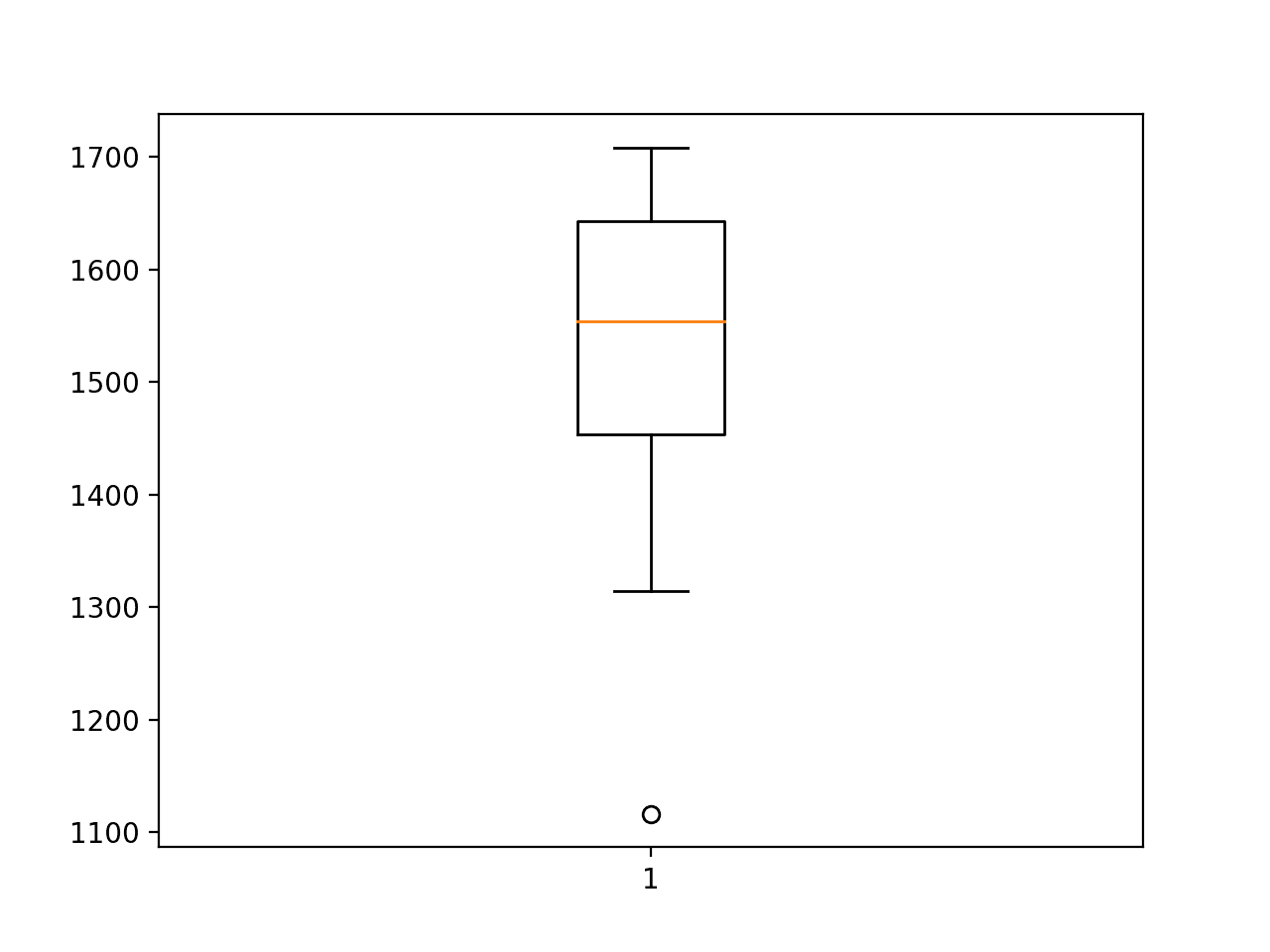
Box and Whisker Plot of Multilayer Perceptron RMSE Forecasting Car Sales
Convolutional Neural Network Model
Convolutional Neural Networks, or CNNs, are a type of neural network developed for two-dimensional image data, although they can be used for one-dimensional data such as sequences of text and time series.
When operating on one-dimensional data, the CNN reads across a sequence of lag observations and learns to extract features that are relevant for making a prediction.
We will define a CNN with two convolutional layers for extracting features from the input sequences. Each will have a configurable number of filters and kernel size and will use the rectified linear activation function. The number of filters determines the number of parallel fields on which the weighted inputs are read and projected. The kernel size defines the number of time steps read within each snapshot as the network reads along the input sequence.
|
1 2 |
model.add(Conv1D(filters=n_filters, kernel_size=n_kernel, activation='relu', input_shape=(n_input, 1))) model.add(Conv1D(filters=n_filters, kernel_size=n_kernel, activation='relu')) |
A max pooling layer is used after convolutional layers to distill the weighted input features into those that are most salient, reducing the input size by 1/4. The pooled inputs are flattened to one long vector before being interpreted and used to make a one-step prediction.
|
1 2 3 |
model.add(MaxPooling1D(pool_size=2)) model.add(Flatten()) model.add(Dense(1)) |
The CNN model expects input data to be in the form of multiple samples, where each sample has multiple input time steps, the same as the MLP in the previous section.
One difference is that the CNN can support multiple features or types of observations at each time step, which are interpreted as channels of an image. We only have a single feature at each time step, therefore the required three-dimensional shape of the input data will be [n_samples, n_input, 1].
|
1 |
train_x = train_x.reshape((train_x.shape[0], train_x.shape[1], 1)) |
The model_fit() function for fitting the CNN model on the training dataset is listed below.
The model takes the following five configuration parameters as a list:
- n_input: The number of lag observations to use as input to the model.
- n_filters: The number of parallel filters.
- n_kernel: The number of time steps considered in each read of the input sequence.
- n_epochs: The number of times to expose the model to the whole training dataset.
- n_batch: The number of samples within an epoch after which the weights are updated.
|
1 2 3 4 5 6 7 8 9 10 11 12 13 14 15 16 17 18 19 |
# fit a model def model_fit(train, config): # unpack config n_input, n_filters, n_kernel, n_epochs, n_batch = config # prepare data data = series_to_supervised(train, n_in=n_input) train_x, train_y = data[:, :-1], data[:, -1] train_x = train_x.reshape((train_x.shape[0], train_x.shape[1], 1)) # define model model = Sequential() model.add(Conv1D(filters=n_filters, kernel_size=n_kernel, activation='relu', input_shape=(n_input, 1))) model.add(Conv1D(filters=n_filters, kernel_size=n_kernel, activation='relu')) model.add(MaxPooling1D(pool_size=2)) model.add(Flatten()) model.add(Dense(1)) model.compile(loss='mse', optimizer='adam') # fit model.fit(train_x, train_y, epochs=n_epochs, batch_size=n_batch, verbose=0) return model |
Making a prediction with the fit CNN model is very much like making a prediction with the fit MLP model in the previous section.
The one difference is in the requirement that we specify the number of features observed at each time step, which in this case is 1. Therefore, when making a single one-step prediction, the shape of the input array must be:
|
1 |
[1, n_input, 1] |
The model_predict() function below implements this behavior.
|
1 2 3 4 5 6 7 8 9 |
# forecast with a pre-fit model def model_predict(model, history, config): # unpack config n_input, _, _, _, _ = config # prepare data x_input = array(history[-n_input:]).reshape((1, n_input, 1)) # forecast yhat = model.predict(x_input, verbose=0) return yhat[0] |
A simple grid search of model hyperparameters was performed and the configuration below was chosen. This is not an optimal configuration, but is the best that was found.
The chosen configuration is as follows:
- n_input: 36 (e.g. 3 years or 3 * 12)
- n_filters: 256
- n_kernel: 3
- n_epochs: 100
- n_batch: 100 (e.g. batch gradient descent)
This can be specified as a list as follows:
|
1 2 |
# define config config = [36, 256, 3, 100, 100] |
Tying all of this together, the complete example is listed below.
|
1 2 3 4 5 6 7 8 9 10 11 12 13 14 15 16 17 18 19 20 21 22 23 24 25 26 27 28 29 30 31 32 33 34 35 36 37 38 39 40 41 42 43 44 45 46 47 48 49 50 51 52 53 54 55 56 57 58 59 60 61 62 63 64 65 66 67 68 69 70 71 72 73 74 75 76 77 78 79 80 81 82 83 84 85 86 87 88 89 90 91 92 93 94 95 96 97 98 99 100 101 102 103 104 105 106 107 108 109 110 111 112 113 114 115 116 117 |
# evaluate cnn from math import sqrt from numpy import array from numpy import mean from numpy import std from pandas import DataFrame from pandas import concat from pandas import read_csv from sklearn.metrics import mean_squared_error from keras.models import Sequential from keras.layers import Dense from keras.layers import Flatten from keras.layers.convolutional import Conv1D from keras.layers.convolutional import MaxPooling1D from matplotlib import pyplot # split a univariate dataset into train/test sets def train_test_split(data, n_test): return data[:-n_test], data[-n_test:] # transform list into supervised learning format def series_to_supervised(data, n_in=1, n_out=1): df = DataFrame(data) cols = list() # input sequence (t-n, ... t-1) for i in range(n_in, 0, -1): cols.append(df.shift(i)) # forecast sequence (t, t+1, ... t+n) for i in range(0, n_out): cols.append(df.shift(-i)) # put it all together agg = concat(cols, axis=1) # drop rows with NaN values agg.dropna(inplace=True) return agg.values # root mean squared error or rmse def measure_rmse(actual, predicted): return sqrt(mean_squared_error(actual, predicted)) # fit a model def model_fit(train, config): # unpack config n_input, n_filters, n_kernel, n_epochs, n_batch = config # prepare data data = series_to_supervised(train, n_in=n_input) train_x, train_y = data[:, :-1], data[:, -1] train_x = train_x.reshape((train_x.shape[0], train_x.shape[1], 1)) # define model model = Sequential() model.add(Conv1D(filters=n_filters, kernel_size=n_kernel, activation='relu', input_shape=(n_input, 1))) model.add(Conv1D(filters=n_filters, kernel_size=n_kernel, activation='relu')) model.add(MaxPooling1D(pool_size=2)) model.add(Flatten()) model.add(Dense(1)) model.compile(loss='mse', optimizer='adam') # fit model.fit(train_x, train_y, epochs=n_epochs, batch_size=n_batch, verbose=0) return model # forecast with a pre-fit model def model_predict(model, history, config): # unpack config n_input, _, _, _, _ = config # prepare data x_input = array(history[-n_input:]).reshape((1, n_input, 1)) # forecast yhat = model.predict(x_input, verbose=0) return yhat[0] # walk-forward validation for univariate data def walk_forward_validation(data, n_test, cfg): predictions = list() # split dataset train, test = train_test_split(data, n_test) # fit model model = model_fit(train, cfg) # seed history with training dataset history = [x for x in train] # step over each time-step in the test set for i in range(len(test)): # fit model and make forecast for history yhat = model_predict(model, history, cfg) # store forecast in list of predictions predictions.append(yhat) # add actual observation to history for the next loop history.append(test[i]) # estimate prediction error error = measure_rmse(test, predictions) print(' > %.3f' % error) return error # repeat evaluation of a config def repeat_evaluate(data, config, n_test, n_repeats=30): # fit and evaluate the model n times scores = [walk_forward_validation(data, n_test, config) for _ in range(n_repeats)] return scores # summarize model performance def summarize_scores(name, scores): # print a summary scores_m, score_std = mean(scores), std(scores) print('%s: %.3f RMSE (+/- %.3f)' % (name, scores_m, score_std)) # box and whisker plot pyplot.boxplot(scores) pyplot.show() series = read_csv('monthly-car-sales.csv', header=0, index_col=0) data = series.values # data split n_test = 12 # define config config = [36, 256, 3, 100, 100] # grid search scores = repeat_evaluate(data, config, n_test) # summarize scores summarize_scores('cnn', scores) |
Running the example first prints the RMSE for each repeated evaluation of the model.
Note: Your results may vary given the stochastic nature of the algorithm or evaluation procedure, or differences in numerical precision. Consider running the example a few times and compare the average outcome.
At the end of the run, we can see that indeed the model is skillful, achieving an average RMSE of 1,524.067, which is better than the naive model, the SARIMA model, and even the MLP model in the previous section.
This is impressive given that the model operated on the raw data directly without scaling or the data being made stationary.
The standard deviation of the score is large, at about 57 sales, but is 1/3 the size of the variance observed with the MLP model in the previous section. We have some confidence that in a bad-case scenario (3 standard deviations), the model RMSE will remain below (better than) the performance of the naive model.
|
1 2 3 4 5 6 7 8 9 10 11 12 13 14 15 16 17 18 19 20 21 22 23 24 25 26 27 28 29 30 31 |
> 1551.031 > 1495.743 > 1449.408 > 1526.017 > 1466.118 > 1566.535 > 1649.204 > 1455.782 > 1574.214 > 1541.790 > 1489.140 > 1506.035 > 1513.197 > 1530.714 > 1511.328 > 1471.518 > 1555.596 > 1552.026 > 1531.727 > 1472.978 > 1620.242 > 1424.153 > 1456.393 > 1581.114 > 1539.286 > 1489.795 > 1652.620 > 1537.349 > 1443.777 > 1567.179 cnn: 1524.067 RMSE (+/- 57.148) |
A box and whisker plot of the scores is created to help understand the spread of error across the runs.
We can see that the spread does seem to be biased towards larger error values, as we would expect, although the upper whisker of the plot (in this case, the largest error that are not outliers) is still limited at an RMSE of 1,650 sales.
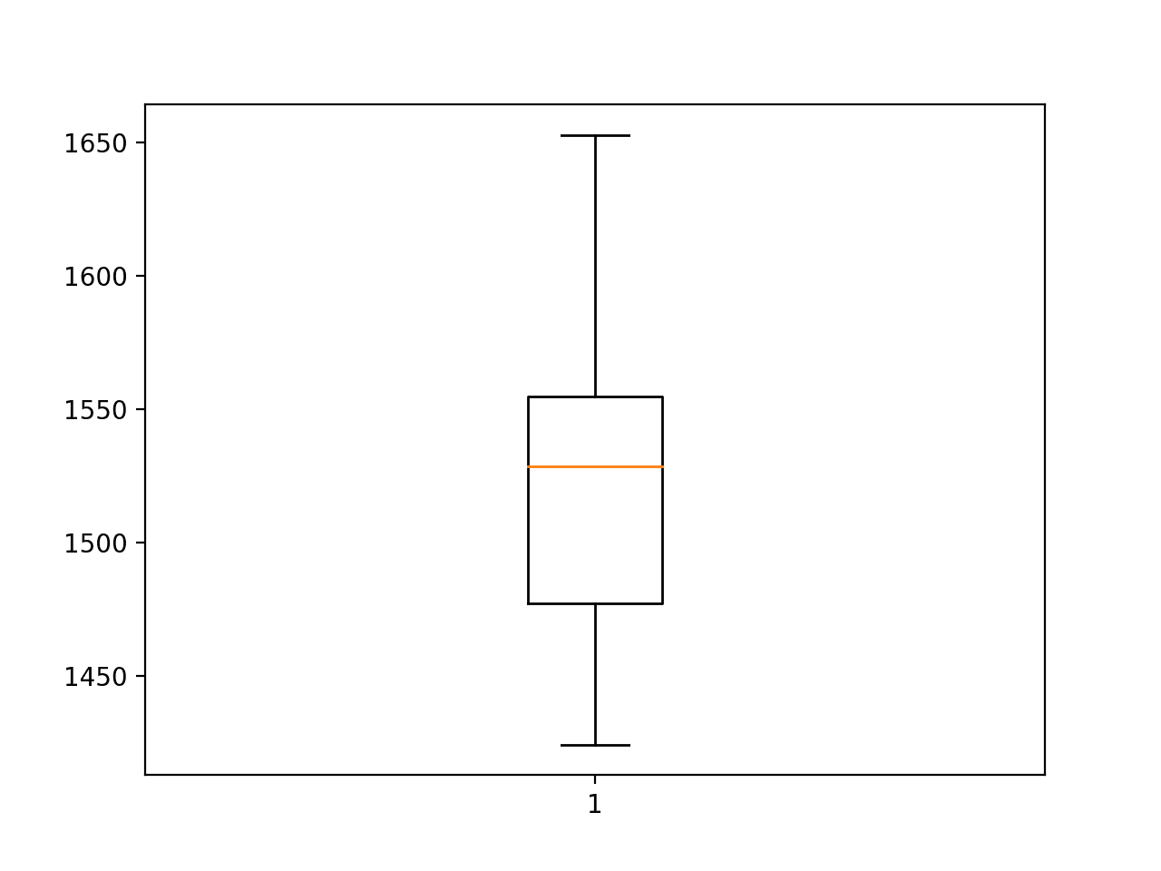
Box and Whisker Plot of Convolutional Neural Network RMSE Forecasting Car Sales
Recurrent Neural Network Models
Recurrent neural networks, or RNNs, are those types of neural networks that use an output of the network from a prior step as an input in attempt to automatically learn across sequence data.
The Long Short-Term Memory, or LSTM, network is a type of RNN whose implementation addresses the general difficulties in training RNNs on sequence data that results in a stable model. It achieves this by learning the weights for internal gates that control the recurrent connections within each node.
Although developed for sequence data, LSTMs have not proven effective on time series forecasting problems where the output is a function of recent observations, e.g. an autoregressive type forecasting problem, such as the car sales dataset.
Nevertheless, we can develop LSTM models for autoregressive problems and use them as a point of comparison with other neural network models.
In this section, we will explore three variations on the LSTM model for univariate time series forecasting; they are:
- LSTM: The LSTM network as-is.
- CNN-LSTM: A CNN network that learns input features and an LSTM that interprets them.
- ConvLSTM: A combination of CNNs and LSTMs where the LSTM units read input data using the convolutional process of a CNN.
LSTM
The LSTM neural network can be used for univariate time series forecasting.
As an RNN, it will read each time step of an input sequence one step at a time. The LSTM has an internal memory allowing it to accumulate internal state as it reads across the steps of a given input sequence.
At the end of the sequence, each node in a layer of hidden LSTM units will output a single value. This vector of values summarizes what the LSTM learned or extracted from the input sequence. This can be interpreted by a fully connected layer before a final prediction is made.
|
1 2 3 4 5 6 |
# define model model = Sequential() model.add(LSTM(n_nodes, activation='relu', input_shape=(n_input, 1))) model.add(Dense(n_nodes, activation='relu')) model.add(Dense(1)) model.compile(loss='mse', optimizer='adam') |
Like the CNN, the LSTM can support multiple variables or features at each time step. As the car sales dataset only has one value at each time step, we can fix this at 1, both when defining the input to the network in the input_shape argument [n_input, 1], and in defining the shape of the input samples.
|
1 |
train_x = train_x.reshape((train_x.shape[0], train_x.shape[1], 1)) |
Unlike the MLP and CNN that do not read the sequence data one-step at a time, the LSTM does perform better if the data is stationary. This means that difference operations are performed to remove the trend and seasonal structure.
In the case of the car sales dataset, we can make the data stationery by performing a seasonal adjustment, that is subtracting the value from one year ago from each observation.
|
1 |
adjusted = value - value[-12] |
This can be performed systematically for the entire training dataset. It also means that the first year of observations must be discarded as we have no prior year of data to difference them with.
The difference() function below will difference a provided dataset with a provided offset, called the difference order, e.g. 12 for one year of months prior.
|
1 2 3 |
# difference dataset def difference(data, interval): return [data[i] - data[i - interval] for i in range(interval, len(data))] |
We can make the difference order a hyperparameter to the model and only perform the operation if a value other than zero is provided.
The model_fit() function for fitting an LSTM model is provided below.
The model expects a list of five model hyperparameters; they are:
- n_input: The number of lag observations to use as input to the model.
- n_nodes: The number of LSTM units to use in the hidden layer.
- n_epochs: The number of times to expose the model to the whole training dataset.
- n_batch: The number of samples within an epoch after which the weights are updated.
- n_diff: The difference order or 0 if not used.
|
1 2 3 4 5 6 7 8 9 10 11 12 13 14 15 16 17 18 19 |
# fit a model def model_fit(train, config): # unpack config n_input, n_nodes, n_epochs, n_batch, n_diff = config # prepare data if n_diff > 0: train = difference(train, n_diff) data = series_to_supervised(train, n_in=n_input) train_x, train_y = data[:, :-1], data[:, -1] train_x = train_x.reshape((train_x.shape[0], train_x.shape[1], 1)) # define model model = Sequential() model.add(LSTM(n_nodes, activation='relu', input_shape=(n_input, 1))) model.add(Dense(n_nodes, activation='relu')) model.add(Dense(1)) model.compile(loss='mse', optimizer='adam') # fit model.fit(train_x, train_y, epochs=n_epochs, batch_size=n_batch, verbose=0) return model |
Making a prediction with the LSTM model is the same as making a prediction with a CNN model.
A single input must have the three-dimensional structure of samples, timesteps, and features, which in this case we only have 1 sample and 1 feature: [1, n_input, 1].
If the difference operation was performed, we must add back the value that was subtracted after the model has made a forecast. We must also difference the historical data prior to formulating the single input used to make a prediction.
The model_predict() function below implements this behavior.
|
1 2 3 4 5 6 7 8 9 10 11 12 13 |
# forecast with a pre-fit model def model_predict(model, history, config): # unpack config n_input, _, _, _, n_diff = config # prepare data correction = 0.0 if n_diff > 0: correction = history[-n_diff] history = difference(history, n_diff) x_input = array(history[-n_input:]).reshape((1, n_input, 1)) # forecast yhat = model.predict(x_input, verbose=0) return correction + yhat[0] |
A simple grid search of model hyperparameters was performed and the configuration below was chosen. This is not an optimal configuration, but is the best that was found.
The chosen configuration is as follows:
- n_input: 36 (i.e. 3 years or 3 * 12)
- n_nodes: 50
- n_epochs: 100
- n_batch: 100 (i.e. batch gradient descent)
- n_diff: 12 (i.e. seasonal difference)
This can be specified as a list:
|
1 2 |
# define config config = [36, 50, 100, 100, 12] |
Tying all of this together, the complete example is listed below.
|
1 2 3 4 5 6 7 8 9 10 11 12 13 14 15 16 17 18 19 20 21 22 23 24 25 26 27 28 29 30 31 32 33 34 35 36 37 38 39 40 41 42 43 44 45 46 47 48 49 50 51 52 53 54 55 56 57 58 59 60 61 62 63 64 65 66 67 68 69 70 71 72 73 74 75 76 77 78 79 80 81 82 83 84 85 86 87 88 89 90 91 92 93 94 95 96 97 98 99 100 101 102 103 104 105 106 107 108 109 110 111 112 113 114 115 116 117 118 119 120 121 122 123 |
# evaluate lstm from math import sqrt from numpy import array from numpy import mean from numpy import std from pandas import DataFrame from pandas import concat from pandas import read_csv from sklearn.metrics import mean_squared_error from keras.models import Sequential from keras.layers import Dense from keras.layers import LSTM from matplotlib import pyplot # split a univariate dataset into train/test sets def train_test_split(data, n_test): return data[:-n_test], data[-n_test:] # transform list into supervised learning format def series_to_supervised(data, n_in=1, n_out=1): df = DataFrame(data) cols = list() # input sequence (t-n, ... t-1) for i in range(n_in, 0, -1): cols.append(df.shift(i)) # forecast sequence (t, t+1, ... t+n) for i in range(0, n_out): cols.append(df.shift(-i)) # put it all together agg = concat(cols, axis=1) # drop rows with NaN values agg.dropna(inplace=True) return agg.values # root mean squared error or rmse def measure_rmse(actual, predicted): return sqrt(mean_squared_error(actual, predicted)) # difference dataset def difference(data, interval): return [data[i] - data[i - interval] for i in range(interval, len(data))] # fit a model def model_fit(train, config): # unpack config n_input, n_nodes, n_epochs, n_batch, n_diff = config # prepare data if n_diff > 0: train = difference(train, n_diff) data = series_to_supervised(train, n_in=n_input) train_x, train_y = data[:, :-1], data[:, -1] train_x = train_x.reshape((train_x.shape[0], train_x.shape[1], 1)) # define model model = Sequential() model.add(LSTM(n_nodes, activation='relu', input_shape=(n_input, 1))) model.add(Dense(n_nodes, activation='relu')) model.add(Dense(1)) model.compile(loss='mse', optimizer='adam') # fit model.fit(train_x, train_y, epochs=n_epochs, batch_size=n_batch, verbose=0) return model # forecast with a pre-fit model def model_predict(model, history, config): # unpack config n_input, _, _, _, n_diff = config # prepare data correction = 0.0 if n_diff > 0: correction = history[-n_diff] history = difference(history, n_diff) x_input = array(history[-n_input:]).reshape((1, n_input, 1)) # forecast yhat = model.predict(x_input, verbose=0) return correction + yhat[0] # walk-forward validation for univariate data def walk_forward_validation(data, n_test, cfg): predictions = list() # split dataset train, test = train_test_split(data, n_test) # fit model model = model_fit(train, cfg) # seed history with training dataset history = [x for x in train] # step over each time-step in the test set for i in range(len(test)): # fit model and make forecast for history yhat = model_predict(model, history, cfg) # store forecast in list of predictions predictions.append(yhat) # add actual observation to history for the next loop history.append(test[i]) # estimate prediction error error = measure_rmse(test, predictions) print(' > %.3f' % error) return error # repeat evaluation of a config def repeat_evaluate(data, config, n_test, n_repeats=30): # fit and evaluate the model n times scores = [walk_forward_validation(data, n_test, config) for _ in range(n_repeats)] return scores # summarize model performance def summarize_scores(name, scores): # print a summary scores_m, score_std = mean(scores), std(scores) print('%s: %.3f RMSE (+/- %.3f)' % (name, scores_m, score_std)) # box and whisker plot pyplot.boxplot(scores) pyplot.show() series = read_csv('monthly-car-sales.csv', header=0, index_col=0) data = series.values # data split n_test = 12 # define config config = [36, 50, 100, 100, 12] # grid search scores = repeat_evaluate(data, config, n_test) # summarize scores summarize_scores('lstm', scores) |
Running the example, we can see the RMSE for each repeated evaluation of the model.
Note: Your results may vary given the stochastic nature of the algorithm or evaluation procedure, or differences in numerical precision. Consider running the example a few times and compare the average outcome.
At the end of the run, we can see that the average RMSE is about 2,109, which is worse than the naive model. This suggests that the chosen model is not skillful, and it was the best that could be found given the same resources used to find model configurations in the previous sections.
This provides further evidence (although weak evidence) that LSTMs, at least alone, are perhaps a bad fit for autoregressive-type sequence prediction problems.
|
1 2 3 4 5 6 7 8 9 10 11 12 13 14 15 16 17 18 19 20 21 22 23 24 25 26 27 28 29 30 31 |
> 2129.480 > 2169.109 > 2078.290 > 2257.222 > 2014.911 > 2197.283 > 2028.176 > 2110.718 > 2100.388 > 2157.271 > 1940.103 > 2086.588 > 1986.696 > 2168.784 > 2188.813 > 2086.759 > 2128.095 > 2126.467 > 2077.463 > 2057.679 > 2209.818 > 2067.082 > 1983.346 > 2157.749 > 2145.071 > 2266.130 > 2105.043 > 2128.549 > 1952.002 > 2188.287 lstm: 2109.779 RMSE (+/- 81.373) |
A box and whisker plot is also created summarizing the distribution of RMSE scores.
Even the base case for the model did not achieve the performance of a naive model.
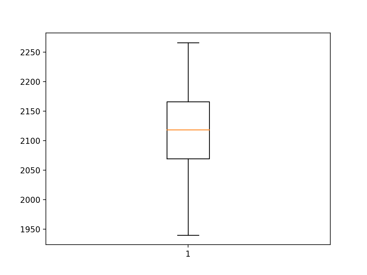
Box and Whisker Plot of Long Short-Term Memory Neural Network RMSE Forecasting Car Sales
CNN LSTM
We have seen that the CNN model is capable of automatically learning and extracting features from the raw sequence data without scaling or differencing.
We can combine this capability with the LSTM where a CNN model is applied to sub-sequences of input data, the results of which together form a time series of extracted features that can be interpreted by an LSTM model.
This combination of a CNN model used to read multiple subsequences over time by an LSTM is called a CNN-LSTM model.
The model requires that each input sequence, e.g. 36 months, is divided into multiple subsequences, each read by the CNN model, e.g. 3 subsequence of 12 time steps. It may make sense to divide the sub-sequences by years, but this is just a hypothesis, and other splits could be used, such as six subsequences of six time steps. Therefore, this splitting is parameterized with the n_seq and n_steps for the number of subsequences and number of steps per subsequence parameters.
|
1 |
train_x = train_x.reshape((train_x.shape[0], n_seq, n_steps, 1)) |
The number of lag observations per sample is simply (n_seq * n_steps).
This is a 4-dimensional input array now with the dimensions:
|
1 |
[samples, subsequences, timesteps, features] |
The same CNN model must be applied to each input subsequence.
We can achieve this by wrapping the entire CNN model in a TimeDistributed layer wrapper.
|
1 2 3 4 5 |
model = Sequential() model.add(TimeDistributed(Conv1D(filters=n_filters, kernel_size=n_kernel, activation='relu', input_shape=(None,n_steps,1)))) model.add(TimeDistributed(Conv1D(filters=n_filters, kernel_size=n_kernel, activation='relu'))) model.add(TimeDistributed(MaxPooling1D(pool_size=2))) model.add(TimeDistributed(Flatten())) |
The output of one application of the CNN submodel will be a vector. The output of the submodel to each input subsequence will be a time series of interpretations that can be interpreted by an LSTM model. This can be followed by a fully connected layer to interpret the outcomes of the LSTM and finally an output layer for making one-step predictions.
|
1 2 3 |
model.add(LSTM(n_nodes, activation='relu')) model.add(Dense(n_nodes, activation='relu')) model.add(Dense(1)) |
The complete model_fit() function is listed below.
The model expects a list of seven hyperparameters; they are:
- n_seq: The number of subsequences within a sample.
- n_steps: The number of time steps within each subsequence.
- n_filters: The number of parallel filters.
- n_kernel: The number of time steps considered in each read of the input sequence.
- n_nodes: The number of LSTM units to use in the hidden layer.
- n_epochs: The number of times to expose the model to the whole training dataset.
- n_batch: The number of samples within an epoch after which the weights are updated.
|
1 2 3 4 5 6 7 8 9 10 11 12 13 14 15 16 17 18 19 20 21 22 |
# fit a model def model_fit(train, config): # unpack config n_seq, n_steps, n_filters, n_kernel, n_nodes, n_epochs, n_batch = config n_input = n_seq * n_steps # prepare data data = series_to_supervised(train, n_in=n_input) train_x, train_y = data[:, :-1], data[:, -1] train_x = train_x.reshape((train_x.shape[0], n_seq, n_steps, 1)) # define model model = Sequential() model.add(TimeDistributed(Conv1D(filters=n_filters, kernel_size=n_kernel, activation='relu', input_shape=(None,n_steps,1)))) model.add(TimeDistributed(Conv1D(filters=n_filters, kernel_size=n_kernel, activation='relu'))) model.add(TimeDistributed(MaxPooling1D(pool_size=2))) model.add(TimeDistributed(Flatten())) model.add(LSTM(n_nodes, activation='relu')) model.add(Dense(n_nodes, activation='relu')) model.add(Dense(1)) model.compile(loss='mse', optimizer='adam') # fit model.fit(train_x, train_y, epochs=n_epochs, batch_size=n_batch, verbose=0) return model |
Making a prediction with the fit model is much the same as the LSTM or CNN, although with the addition of splitting each sample into subsequences with a given number of time steps.
|
1 2 |
# prepare data x_input = array(history[-n_input:]).reshape((1, n_seq, n_steps, 1)) |
The updated model_predict() function is listed below.
|
1 2 3 4 5 6 7 8 9 10 |
# forecast with a pre-fit model def model_predict(model, history, config): # unpack config n_seq, n_steps, _, _, _, _, _ = config n_input = n_seq * n_steps # prepare data x_input = array(history[-n_input:]).reshape((1, n_seq, n_steps, 1)) # forecast yhat = model.predict(x_input, verbose=0) return yhat[0] |
A simple grid search of model hyperparameters was performed and the configuration below was chosen. This may not be an optimal configuration, but it is the best that was found.
- n_seq: 3 (i.e. 3 years)
- n_steps: 12 (i.e. 1 year of months)
- n_filters: 64
- n_kernel: 3
- n_nodes: 100
- n_epochs: 200
- n_batch: 100 (i.e. batch gradient descent)
We can define the configuration as a list; for example:
|
1 2 |
# define config config = [3, 12, 64, 3, 100, 200, 100] |
The complete example of evaluating the CNN-LSTM model for forecasting the univariate monthly car sales is listed below.
|
1 2 3 4 5 6 7 8 9 10 11 12 13 14 15 16 17 18 19 20 21 22 23 24 25 26 27 28 29 30 31 32 33 34 35 36 37 38 39 40 41 42 43 44 45 46 47 48 49 50 51 52 53 54 55 56 57 58 59 60 61 62 63 64 65 66 67 68 69 70 71 72 73 74 75 76 77 78 79 80 81 82 83 84 85 86 87 88 89 90 91 92 93 94 95 96 97 98 99 100 101 102 103 104 105 106 107 108 109 110 111 112 113 114 115 116 117 118 119 120 121 122 123 |
# evaluate cnn lstm from math import sqrt from numpy import array from numpy import mean from numpy import std from pandas import DataFrame from pandas import concat from pandas import read_csv from sklearn.metrics import mean_squared_error from keras.models import Sequential from keras.layers import Dense from keras.layers import LSTM from keras.layers import TimeDistributed from keras.layers import Flatten from keras.layers.convolutional import Conv1D from keras.layers.convolutional import MaxPooling1D from matplotlib import pyplot # split a univariate dataset into train/test sets def train_test_split(data, n_test): return data[:-n_test], data[-n_test:] # transform list into supervised learning format def series_to_supervised(data, n_in=1, n_out=1): df = DataFrame(data) cols = list() # input sequence (t-n, ... t-1) for i in range(n_in, 0, -1): cols.append(df.shift(i)) # forecast sequence (t, t+1, ... t+n) for i in range(0, n_out): cols.append(df.shift(-i)) # put it all together agg = concat(cols, axis=1) # drop rows with NaN values agg.dropna(inplace=True) return agg.values # root mean squared error or rmse def measure_rmse(actual, predicted): return sqrt(mean_squared_error(actual, predicted)) # fit a model def model_fit(train, config): # unpack config n_seq, n_steps, n_filters, n_kernel, n_nodes, n_epochs, n_batch = config n_input = n_seq * n_steps # prepare data data = series_to_supervised(train, n_in=n_input) train_x, train_y = data[:, :-1], data[:, -1] train_x = train_x.reshape((train_x.shape[0], n_seq, n_steps, 1)) # define model model = Sequential() model.add(TimeDistributed(Conv1D(filters=n_filters, kernel_size=n_kernel, activation='relu', input_shape=(None,n_steps,1)))) model.add(TimeDistributed(Conv1D(filters=n_filters, kernel_size=n_kernel, activation='relu'))) model.add(TimeDistributed(MaxPooling1D(pool_size=2))) model.add(TimeDistributed(Flatten())) model.add(LSTM(n_nodes, activation='relu')) model.add(Dense(n_nodes, activation='relu')) model.add(Dense(1)) model.compile(loss='mse', optimizer='adam') # fit model.fit(train_x, train_y, epochs=n_epochs, batch_size=n_batch, verbose=0) return model # forecast with a pre-fit model def model_predict(model, history, config): # unpack config n_seq, n_steps, _, _, _, _, _ = config n_input = n_seq * n_steps # prepare data x_input = array(history[-n_input:]).reshape((1, n_seq, n_steps, 1)) # forecast yhat = model.predict(x_input, verbose=0) return yhat[0] # walk-forward validation for univariate data def walk_forward_validation(data, n_test, cfg): predictions = list() # split dataset train, test = train_test_split(data, n_test) # fit model model = model_fit(train, cfg) # seed history with training dataset history = [x for x in train] # step over each time-step in the test set for i in range(len(test)): # fit model and make forecast for history yhat = model_predict(model, history, cfg) # store forecast in list of predictions predictions.append(yhat) # add actual observation to history for the next loop history.append(test[i]) # estimate prediction error error = measure_rmse(test, predictions) print(' > %.3f' % error) return error # repeat evaluation of a config def repeat_evaluate(data, config, n_test, n_repeats=30): # fit and evaluate the model n times scores = [walk_forward_validation(data, n_test, config) for _ in range(n_repeats)] return scores # summarize model performance def summarize_scores(name, scores): # print a summary scores_m, score_std = mean(scores), std(scores) print('%s: %.3f RMSE (+/- %.3f)' % (name, scores_m, score_std)) # box and whisker plot pyplot.boxplot(scores) pyplot.show() series = read_csv('monthly-car-sales.csv', header=0, index_col=0) data = series.values # data split n_test = 12 # define config config = [3, 12, 64, 3, 100, 200, 100] # grid search scores = repeat_evaluate(data, config, n_test) # summarize scores summarize_scores('cnn-lstm', scores) |
Running the example prints the RMSE for each repeated evaluation of the model.
Note: Your results may vary given the stochastic nature of the algorithm or evaluation procedure, or differences in numerical precision. Consider running the example a few times and compare the average outcome.
The final averaged RMSE is reported at the end of about 1,626, which is lower than the naive model, but still higher than a SARIMA model. The standard deviation of this score is also very large, suggesting that the chosen configuration may not be as stable as the standalone CNN model.
|
1 2 3 4 5 6 7 8 9 10 11 12 13 14 15 16 17 18 19 20 21 22 23 24 25 26 27 28 29 30 31 |
> 1543.533 > 1421.895 > 1467.927 > 1441.125 > 1750.995 > 1321.498 > 1571.657 > 1845.298 > 1621.589 > 1425.065 > 1675.232 > 1807.288 > 2922.295 > 1391.861 > 1626.655 > 1633.177 > 1667.572 > 1577.285 > 1590.235 > 1557.385 > 1784.982 > 1664.839 > 1741.729 > 1437.992 > 1772.076 > 1289.794 > 1685.976 > 1498.123 > 1618.627 > 1448.361 cnn-lstm: 1626.735 RMSE (+/- 279.850) |
A box and whisker plot is also created summarizing the distribution of RMSE scores.
The plot shows one single outlier of very poor performance just below 3,000 sales.
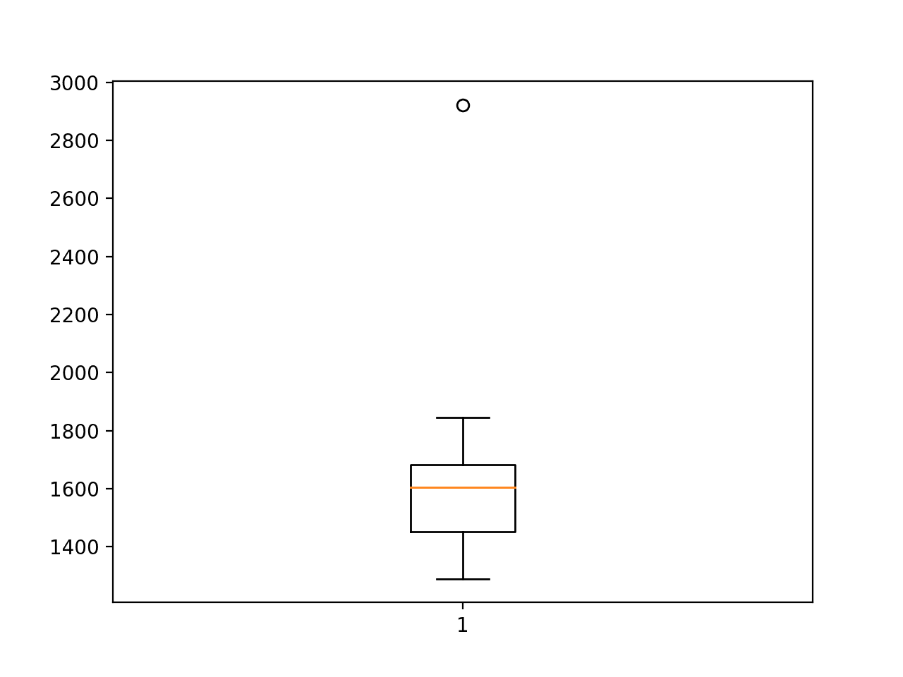
Box and Whisker Plot of CNN-LSTM RMSE Forecasting Car Sales
ConvLSTM
It is possible to perform a convolutional operation as part of the read of the input sequence within each LSTM unit.
This means, rather than reading a sequence one step at a time, the LSTM would read a block or subsequence of observations at a time using a convolutional process, like a CNN.
This is different to first reading an extracting features with an LSTM and interpreting the result with an LSTM; this is performing the CNN operation at each time step as part of the LSTM.
This type of model is called a Convolutional LSTM, or ConvLSTM for short. It is provided in Keras as a layer called ConvLSTM2D for 2D data. We can configure it for use with 1D sequence data by assuming that we have one row with multiple columns.
As with the CNN-LSTM, the input data is split into subsequences where each subsequence has a fixed number of time steps, although we must also specify the number of rows in each subsequence, which in this case is fixed at 1.
|
1 |
train_x = train_x.reshape((train_x.shape[0], n_seq, 1, n_steps, 1)) |
The shape is five-dimensional, with the dimensions:
|
1 |
[samples, subsequences, rows, columns, features] |
Like the CNN, the ConvLSTM layer allows us to specify the number of filter maps and the size of the kernel used when reading the input sequences.
|
1 |
model.add(ConvLSTM2D(filters=n_filters, kernel_size=(1,n_kernel), activation='relu', input_shape=(n_seq, 1, n_steps, 1))) |
The output of the layer is a sequence of filter maps that must first be flattened before it can be interpreted and followed by an output layer.
The model expects a list of seven hyperparameters, the same as the CNN-LSTM; they are:
- n_seq: The number of subsequences within a sample.
- n_steps: The number of time steps within each subsequence.
- n_filters: The number of parallel filters.
- n_kernel: The number of time steps considered in each read of the input sequence.
- n_nodes: The number of LSTM units to use in the hidden layer.
- n_epochs: The number of times to expose the model to the whole training dataset.
- n_batch: The number of samples within an epoch after which the weights are updated.
The model_fit() function that implements all of this is listed below.
|
1 2 3 4 5 6 7 8 9 10 11 12 13 14 15 16 17 18 19 |
# fit a model def model_fit(train, config): # unpack config n_seq, n_steps, n_filters, n_kernel, n_nodes, n_epochs, n_batch = config n_input = n_seq * n_steps # prepare data data = series_to_supervised(train, n_in=n_input) train_x, train_y = data[:, :-1], data[:, -1] train_x = train_x.reshape((train_x.shape[0], n_seq, 1, n_steps, 1)) # define model model = Sequential() model.add(ConvLSTM2D(filters=n_filters, kernel_size=(1,n_kernel), activation='relu', input_shape=(n_seq, 1, n_steps, 1))) model.add(Flatten()) model.add(Dense(n_nodes, activation='relu')) model.add(Dense(1)) model.compile(loss='mse', optimizer='adam') # fit model.fit(train_x, train_y, epochs=n_epochs, batch_size=n_batch, verbose=0) return model |
A prediction is made with the fit model in the same way as the CNN-LSTM, although with the additional rows dimension that we fix to 1.
|
1 2 |
# prepare data x_input = array(history[-n_input:]).reshape((1, n_seq, 1, n_steps, 1)) |
The model_predict() function for making a single one-step prediction is listed below.
|
1 2 3 4 5 6 7 8 9 10 |
# forecast with a pre-fit model def model_predict(model, history, config): # unpack config n_seq, n_steps, _, _, _, _, _ = config n_input = n_seq * n_steps # prepare data x_input = array(history[-n_input:]).reshape((1, n_seq, 1, n_steps, 1)) # forecast yhat = model.predict(x_input, verbose=0) return yhat[0] |
A simple grid search of model hyperparameters was performed and the configuration below was chosen.
This may not be an optimal configuration, but is the best that was found.
- n_seq: 3 (i.e. 3 years)
- n_steps: 12 (i.e. 1 year of months)
- n_filters: 256
- n_kernel: 3
- n_nodes: 200
- n_epochs: 200
- n_batch: 100 (i.e. batch gradient descent)
We can define the configuration as a list; for example:
|
1 2 |
# define config config = [3, 12, 256, 3, 200, 200, 100] |
We can tie all of this together. The complete code listing for the ConvLSTM model evaluated for one-step forecasting of the monthly car sales dataset is listed below.
|
1 2 3 4 5 6 7 8 9 10 11 12 13 14 15 16 17 18 19 20 21 22 23 24 25 26 27 28 29 30 31 32 33 34 35 36 37 38 39 40 41 42 43 44 45 46 47 48 49 50 51 52 53 54 55 56 57 58 59 60 61 62 63 64 65 66 67 68 69 70 71 72 73 74 75 76 77 78 79 80 81 82 83 84 85 86 87 88 89 90 91 92 93 94 95 96 97 98 99 100 101 102 103 104 105 106 107 108 109 110 111 112 113 114 115 116 117 118 119 120 121 |
# evaluate convlstm from math import sqrt from numpy import array from numpy import mean from numpy import std from pandas import DataFrame from pandas import concat from pandas import read_csv from sklearn.metrics import mean_squared_error from keras.models import Sequential from keras.layers import Dense from keras.layers import Flatten from keras.layers import ConvLSTM2D from matplotlib import pyplot # split a univariate dataset into train/test sets def train_test_split(data, n_test): return data[:-n_test], data[-n_test:] # transform list into supervised learning format def series_to_supervised(data, n_in=1, n_out=1): df = DataFrame(data) cols = list() # input sequence (t-n, ... t-1) for i in range(n_in, 0, -1): cols.append(df.shift(i)) # forecast sequence (t, t+1, ... t+n) for i in range(0, n_out): cols.append(df.shift(-i)) # put it all together agg = concat(cols, axis=1) # drop rows with NaN values agg.dropna(inplace=True) return agg.values # root mean squared error or rmse def measure_rmse(actual, predicted): return sqrt(mean_squared_error(actual, predicted)) # difference dataset def difference(data, interval): return [data[i] - data[i - interval] for i in range(interval, len(data))] # fit a model def model_fit(train, config): # unpack config n_seq, n_steps, n_filters, n_kernel, n_nodes, n_epochs, n_batch = config n_input = n_seq * n_steps # prepare data data = series_to_supervised(train, n_in=n_input) train_x, train_y = data[:, :-1], data[:, -1] train_x = train_x.reshape((train_x.shape[0], n_seq, 1, n_steps, 1)) # define model model = Sequential() model.add(ConvLSTM2D(filters=n_filters, kernel_size=(1,n_kernel), activation='relu', input_shape=(n_seq, 1, n_steps, 1))) model.add(Flatten()) model.add(Dense(n_nodes, activation='relu')) model.add(Dense(1)) model.compile(loss='mse', optimizer='adam') # fit model.fit(train_x, train_y, epochs=n_epochs, batch_size=n_batch, verbose=0) return model # forecast with a pre-fit model def model_predict(model, history, config): # unpack config n_seq, n_steps, _, _, _, _, _ = config n_input = n_seq * n_steps # prepare data x_input = array(history[-n_input:]).reshape((1, n_seq, 1, n_steps, 1)) # forecast yhat = model.predict(x_input, verbose=0) return yhat[0] # walk-forward validation for univariate data def walk_forward_validation(data, n_test, cfg): predictions = list() # split dataset train, test = train_test_split(data, n_test) # fit model model = model_fit(train, cfg) # seed history with training dataset history = [x for x in train] # step over each time-step in the test set for i in range(len(test)): # fit model and make forecast for history yhat = model_predict(model, history, cfg) # store forecast in list of predictions predictions.append(yhat) # add actual observation to history for the next loop history.append(test[i]) # estimate prediction error error = measure_rmse(test, predictions) print(' > %.3f' % error) return error # repeat evaluation of a config def repeat_evaluate(data, config, n_test, n_repeats=30): # fit and evaluate the model n times scores = [walk_forward_validation(data, n_test, config) for _ in range(n_repeats)] return scores # summarize model performance def summarize_scores(name, scores): # print a summary scores_m, score_std = mean(scores), std(scores) print('%s: %.3f RMSE (+/- %.3f)' % (name, scores_m, score_std)) # box and whisker plot pyplot.boxplot(scores) pyplot.show() series = read_csv('monthly-car-sales.csv', header=0, index_col=0) data = series.values # data split n_test = 12 # define config config = [3, 12, 256, 3, 200, 200, 100] # grid search scores = repeat_evaluate(data, config, n_test) # summarize scores summarize_scores('convlstm', scores) |
Running the example prints the RMSE for each repeated evaluation of the model.
Note: Your results may vary given the stochastic nature of the algorithm or evaluation procedure, or differences in numerical precision. Consider running the example a few times and compare the average outcome.
The final averaged RMSE is reported at the end of about 1,660, which is lower than the naive model, but still higher than a SARIMA model.
It is a result that is perhaps on par with the CNN-LSTM model. The standard deviation of this score is also very large, suggesting that the chosen configuration may not be as stable as the standalone CNN model.
|
1 2 3 4 5 6 7 8 9 10 11 12 13 14 15 16 17 18 19 20 21 22 23 24 25 26 27 28 29 30 31 |
> 1825.246 > 1862.674 > 1684.313 > 1310.448 > 2109.668 > 1507.912 > 1431.118 > 1442.692 > 1400.548 > 1732.381 > 1523.824 > 1611.898 > 1805.970 > 1616.015 > 1649.466 > 1521.884 > 2025.655 > 1622.886 > 2536.448 > 1526.532 > 1866.631 > 1562.625 > 1491.386 > 1506.270 > 1843.981 > 1653.084 > 1650.430 > 1291.353 > 1558.616 > 1653.231 convlstm: 1660.840 RMSE (+/- 248.826) |
A box and whisker plot is also created, summarizing the distribution of RMSE scores.
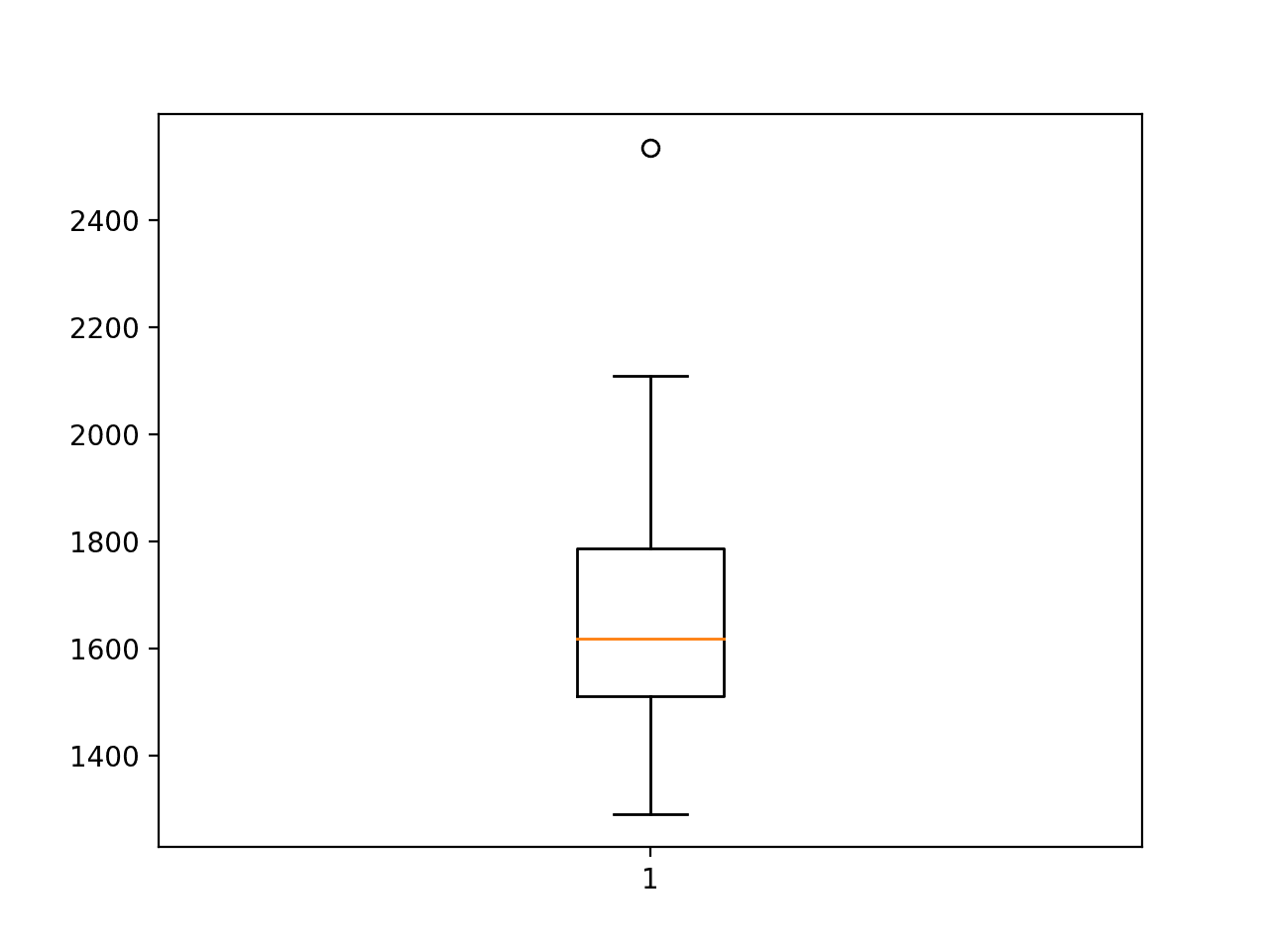
Box and Whisker Plot of ConvLSTM RMSE Forecasting Car Sales
Extensions
This section lists some ideas for extending the tutorial that you may wish to explore.
- Data Preparation. Explore whether data preparation, such as normalization, standardization, and/or differencing can list the performance of any of the models.
- Grid Search Hyperparameters. Implement a grid search of the hyperparameters for one model to see if you can further lift performance.
- Learning Curve Diagnostics. Create a single fit of one model and review the learning curves on train and validation splits of the dataset, then use the diagnostics of the learning curves to further tune the model hyperparameters in order to improve model performance.
- History Size. Explore different amounts of historical data (lag inputs) for one model to see if you can further improve model performance
- Reduce Variance of Final Model. Explore one or more strategies to reduce the variance for one of the neural network models.
- Update During Walk-Forward. Explore whether re-fitting or updating a neural network model as part of walk-forward validation can further improve model performance.
- More Parameterization. Explore adding further model parameterization for one model, such as the use of additional layers.
If you explore any of these extensions, I’d love to know.
Further Reading
This section provides more resources on the topic if you are looking to go deeper.
- pandas.DataFrame.shift API
- sklearn.metrics.mean_squared_error API
- matplotlib.pyplot.boxplot API
- Keras Sequence Model API
Summary
In this tutorial, you discovered how to develop a suite of deep learning models for univariate time series forecasting.
Specifically, you learned:
- How to develop a robust test harness using walk-forward validation for evaluating the performance of neural network models.
- How to develop and evaluate simple multilayer Perceptron and convolutional neural networks for time series forecasting.
- How to develop and evaluate LSTMs, CNN-LSTMs, and ConvLSTM neural network models for time series forecasting.
Do you have any questions?
Ask your questions in the comments below and I will do my best to answer.
Develop Deep Learning models for Time Series Today!

Develop Your Own Forecasting models in Minutes
...with just a few lines of python code
Discover how in my new Ebook:
Deep Learning for Time Series Forecasting
It provides self-study tutorials on topics like:
CNNs, LSTMs,
Multivariate Forecasting, Multi-Step Forecasting and much more...
Finally Bring Deep Learning to your Time Series Forecasting Projects
Skip the Academics. Just Results.


")
Hello . Andy. Ukraine. Kiev.
In your example CNN LSTM (whole code model) I have error.
File “C:\Users\User\Dropbox\DeepLearning3\realmodproj\project\educationNew\sub2\step_005.py”, line 89, in model_fit
model.add(TimeDistributed(Conv1D(filters=n_filters, kernel_size=n_kernel, activation=’relu’, input_shape=(None,n_steps,1))))
File “C:\Users\User\AppData\Local\Programs\Python\Python36\lib\site-packages\keras\models.py”, line 454, in add
raise ValueError(‘The first layer in a ‘
ValueError: The first layer in a Sequential model must get an
input_shapeorbatch_input_shapeargument.Coud you explame me what the reason ?
Thank you.
I believe you need to update your version of Keras to 2.2.4 or higher.
Using TensorFlow backend.
1.8.0
I recommend using tensorflow 1.11.0 or higher.
Andy , Kiev
May be i should use ?
model.add(TimeDistributed( Conv1D(filters=n_filters, kernel_size=n_kernel, activation=’relu’, input_shape=(None,n_steps,1) ) , input_shape=(None,n_steps,1) ) )
Sure, that was required for older versions of Keras.
So, in a nutshell, RNN doesn’t work very well when dealing with time series forecasting?
Correct, they will be outperformed by linear methods on univariate data in most cases.
Also see this:
https://machinelearningmastery.com/findings-comparing-classical-and-machine-learning-methods-for-time-series-forecasting/
Thanks for the article
I have a univariate time series classification problem. Data comes from the accelerometer sensor (vibration analysis). only X-axis. and the sampling rate is 2.5 KHz and I need a real-time classification.
what’s your suggestion for classifying this time series? I want to differentiate between multiple labeled classes (failures).
which of your articles can help me? I read all of them but many of them are not univariate and this article which is univariate is about forecasting and not classification.
thanks indeed.
Sounds like time series classification.
You could look at the HAR articles, for example:
https://machinelearningmastery.com/how-to-develop-rnn-models-for-human-activity-recognition-time-series-classification/
Hi Jason and thanks for all of your amazing turorials on ML!
I am new to time-series forecasting, but I have been learning a lot from your articles.
I have a issue were am trying to forecast the amount of tickets sold per day, but I would like to the forecast 60 days before the actual date. I have 3 years of historical data on the tickets sold per day.
Testing the above models on my data, the persistence model scored the best (I think) with a 4.041 RMSE, the next best was the MLP with 7.501 (+/- 0.589) RMSE.
Do you have any recommendation on how to proceed doing the forecast for my data?
Thanks again for your great work!
Nice work.
Yes, what is the problem that you are having exactly?
Hey,
Say I have show, and 60 days before the show I want to forecast how many tickets sold during those 60days.(t+60)
If I look at the the 60days as one time period, the forecast would not consider seasonal effects, which have a big effect on the tickets sold. Therfore, I think I need to use each day during those 60 days as a period for a more accurate forecast.
So, I want to forecast the tickest sold each day during a 60 day period, but I want to know the forecast before that 60 day period starts. And the output of the model is a list of 60 elements representing the expected ticket sale for each day [0,1,7,5,3…,3]
My problem is choosing the correct approach for such forecast. Do you have any tips?
That sounds like a very challenging problem.
We cannot know the best approach. You must discover the best approach through experimentation with a suite of different methods.
This might help:
https://machinelearningmastery.com/how-to-develop-a-skilful-time-series-forecasting-model/
your blog pretty good
Thanks.
Thank you for the code and explanation. I am working on a univariate time series data for forecasting. I have 60 data points or basically 5-years data in months. If I want to predict the last year or the last 12 months, will my n_test = 12 ? and I was wondering how to see the last 12 predictions made my the model so I can graph the actual with predicted ?.
Thank You.
It sounds like you want to make a multi-step forecast. I give a number of examples here:
https://machinelearningmastery.com/start-here/#deep_learning_time_series
Appreciate you so much about posting valuable article!!!!
Thanks!~~~
Oh I have a quick question. Why does rmse score change every time repeating evaluation although config or hyper params are not adjusted?
Good question, I answer it here:
https://machinelearningmastery.com/faq/single-faq/why-do-i-get-different-results-each-time-i-run-the-code
You’re welcome, I’m glad it helped.
is it possible to use “ensemble methods” machine learning (such as bagging, boosting ..) for the forecasting?
If so, when and how?
Can you lead me to an example of time series forecasting with ensemble methods
thank you in advance
Yes, you can get started here:
https://machinelearningmastery.com/start-here/#deep_learning_time_series
And here:
https://machinelearningmastery.com/start-here/#better
thank you sir
I don’t think that’s for time series forecasting!
Thank you for these explanations.
How can we add a confidence interval for the prediction.
I think you mean prediction interval:
https://machinelearningmastery.com/prediction-intervals-for-machine-learning/
Hi Jason, thank you so much for this article, it helps me a lot. Could you attach the link of articles you used naive method and SARIMA to do forecasting on the monthly sales data set? I searched your articles but didn’t find them. Thanks!
You can use the search box at the top of the page, e.g. “naive bayes” or “sarima”.
Hi Jason, thank you so much for your last reply. I was using your models to fit a time series data of total demand quantity each week for a product, and I found that the RMSE of CNN-LSTM varies a lot. Sometimes I got a very good result, in which the RSME is half of that of MLP model, sometimes I got just-so-so result, and sometimes I got very bad result, in which the RSME is much more worse than what I got from naive forecasting. Could you tell me some methods to avoid this and only get good results, like how to choose the parameters for CNN-LSTM? Thanks!
Great question.
You can try some regularization methods and perhaps increase the capacity of the model.
I give examples here:
https://machinelearningmastery.com/start-here/#better
Hi Jason, this is really a great tutorial, thanks!
I have one question about the the walk forward validation in deep learning neural network models.
I understood the concept of walk forward validation in models when you wanna make a one step ahead forecast that you compare the prediction with the actual test value and update your window with the true known window from the test set to forecast the next period.
For deep learning models I’m lacking the understanding a little bit. As I see more complex models, such as neural networks, do not refit the model in the ‘typical’ walk forward validation way because of the complexity of computation.
What does the walk forward validation in your MLP code or CNN code means exactly then? That you use true observation as part of the input layer to make a prediction for the next time step?
We use the same walk-forward validation process as we would use with other models.
And what do the X-train and y_ train in the MLP code when you fit the model imply? Maybe that’s the answer to my question that you continuously update the X-train with the forecasted y values?
We can choose to re-fit the model with each new observation, e.g. each step, or not. We typically do not because of the computational expense.
Hi Jason,
In case a dataset with climate variables to predict precipitation using LSTM, and supposing the is not stationary, Can I apply the difference? With 10 years, should I do per year?
Thanks in advance!
André
Try a 1-step difference to remove a trend, try a seasonal difference to remove seasonality.
Hi Jason,
I’m trying to adapt this code to a multivariate approach (LSTM) and couldn’t understand very well the function walk_forward_validation.
You have used the train (data) to fit the model. Why you use the same train data to predict the model on line ‘yhat = model_predict(model, history, cfg)’ ? Why not use the test? And compare with test (real).
I give examples of multivariate forecasting with LSTMs here:
https://machinelearningmastery.com/start-here/#deep_learning_time_series
This might be a good place to start:
https://machinelearningmastery.com/how-to-develop-lstm-models-for-time-series-forecasting/
Hello ! Thanks for this amazing tutorial but I have the same question above and I couldn’t find an answer on the links you proposed.
Why should I feed my predict_model function with the training set (history) ?
Normally, I should give my predict_model function only the x_test part and ask it to calculate the y_hat !
Can you please give us more explanation about that ? Thanks again
You’re welcome.
I think you’re asking about how we are evaluating the performance of the model. In this case, we are using walk-forward validation, a standard technique for evaluating sequence prediction models. You can learn more about it here:
https://machinelearningmastery.com/backtest-machine-learning-models-time-series-forecasting/
Hi, i want to forecast 800 ish products, is it possible to use RNN to forecast those products in one time? or I need to do it one by one?
Great question.
There are many ways, I explain some approaches here (replace “sites” with “products”)
https://machinelearningmastery.com/faq/single-faq/how-to-develop-forecast-models-for-multiple-sites
Hi Jason, since this reply is about one year old, may I know do you still hold this view: Vanilla LSTMs are very poor at time series forecasting… ConvLSTMs are very good?
If yes, do you write any articles (or books) on how to develop ConvLSTMs model?
Why am I asking is that i would like to look for candidate models other than the Bayesian approach (which I think is analytically heavy). Thank you.
Yes, see this study:
https://machinelearningmastery.com/findings-comparing-classical-and-machine-learning-methods-for-time-series-forecasting/
Yes, CNN-LSTMs and ConvLSTMs are covered here:
https://machinelearningmastery.com/how-to-develop-lstm-models-for-time-series-forecasting/
Hello Jason! Thank you very much for giving as an insight of neural network for forecasting. I am dealing with a forecasting problem, where I need to predict 23 days (one month aprox) of production, based on 831 days of former production. I already tested my data, and I realized it is stationary, so LSTM RNN didn’t work in the first time. So, I thought that maybe, a basic MLP could work, and I followed your tutorial. It all went well, but I need now to grab de list o predicted data, for plotting them against the test data, and I am having trouble with the code to do this. Could you please help me? (I am sort of new in all this “deep learning” thing)
Nice work.
Yes, use the model to make the prediction then plot it. e.g.
yhat = model.predict(newX)
If the model predicts 23 time steps directly, then that is all you need.
If you designed the model to predict 1 time step, then call the model 23 times with different inputs required.
Then plot with matplotlib:
pyplot.plot(yhat)
pyplot.show()
I hope that helps.
Hey Jason,
Getting model not defined error. Should I be placing this in the define loop?
Thanks!
“model” is the name of the reference to your model object, whatever that happens to be.
Hi Jason, I have tried the models here and I want to apply them to multi-site data and get the predictions for them at the same time. For example, for the data set you are using here, if I want to predict the monthly sales of cars of different brands, and I want to get the sales forecasts of these brands, what should I do to modify the code? I saw you have a EMC Data Science Global Hackathon data set which is multi-site, but I didn’ t find a model for it. Thanks and have a good weekend!
For my above question, I mean deep learning models for multi-site data. I saw you developed time series model and machine learning models for the air pollution data set.
Good question, I have some suggestions here that might help:
https://machinelearningmastery.com/faq/single-faq/how-to-develop-forecast-models-for-multiple-sites
Hello Dr. Brownlee,
thank you for all the free resources.
I’m doing a IoT based uni project and I need to do some predictions with the dataset.
My created data set:
Hourly decimal values, over the course of a month. (dim 500×1, config = [24, 500, 100, 100, n_test = 0.75)
1) I already tried winter holds & got a RSME of 6.66. I’m aware of your article which states, that analytical approaches are often better then ML approaches. So I tried it with the MLP example & got immediately better results. However I’m not sure wether your RSME calculation is comparable. Whenever the walk-foward-validation method is run, you append the actual “future” value of the test set. Therefore the algorithm only predicts one value in the future. When I changed history.append(test[i]) to history.append(yhat) I got horrible results. Am I all wrong or are the two RSME’s not comparable?
2) How do I predict the future once the algorithm is trained, since the model types are only accessible within the methods?
Otherwise I would just warp a for loop around this:
history = [x for x in data]
x_input = np.array(history[-24:]).reshape(1, 24)
yhat = model.predict(x_input, verbose=0)
print(yhat)
Thanks in advance & have a pleasant day 😉
For apples to apples comparison, both methods must be evaluated under an identical test harness.
If your model is intended to be used for multi-step forecasting, then you should evaluate it that way, rather than one step forecasts.
I hope that helps.
Hello, thank you very much for this post.
I didn’t understand a thing on CNN-LSTM.
I have a database related to parking.
Data is stored every hour and I have 12 data per day.
And I saved this data for 10 months.
I want to use CNN-LSTM, but I don’t know how to set the values of n_seq and n_Step.
Perhaps start with the simple example here and adapt it for your dataset:
https://machinelearningmastery.com/how-to-develop-lstm-models-for-time-series-forecasting/
Thanks.
Is there a specific rule for dividing data into samples in CNN-LSTM?
For example, in your example, there are 108 data. The number of samples in the CNN-LSTM model is 36.
And it’s n_seq =3 and n_step is 12.
Why are these numbers chosen?
Is it possible to have n_seq=5 and its n_step is 20?
What is the reason for choosing these numbers?
I have 1312 data, should the number of samples be 1312 / 3?
1312 / 3 = 437
n_seq = 3
n_step = 437 / n_seq
is it correct?
How do I select the n_seq and n_Steps numbers?
No rules.
Design a test harness that best evaluates your model on your data in a way you expect to use the model in the future.
If you only have about 100 observations, perhaps stick with a linear method like ETS or SARIMA?
Thank you Mr. Jason Brownlee.
In the example you wrote (in CNN-LSTM), you considered each 36 data as input and gave the 37th data as a target.
And that’s why the multiplication of n_seq and n_steps is equal to 36 :
3 * 12 = 36
Now let’s assume that if we have to divide the data into the train and test so that we have 37 data for the input and the 38th data is for the target.
Therefore, the value of n_seq and n_steps cannot be the integer values.
because 12.33 * 3 = 37
And we know that to interpret any sample by cnn we have to divide the sample into several subsequences and step.
What should be done in these cases?
Thanks
You may have to experiment with different division of the dataset set to see what works well. Experiment!
Thank you Jason for such a great example. It will be of great help if you can analyse the same problem using R software.
Thanks for the suggestion.
Thank you for your nice post.
I have a list of date, using this list of date pattern, I want to predict next date.
So how can I do it? I am searching but I am failed. Can you please give me a suggestion?
Thanks
Perhaps convert the dates to integers and try modeling it as a forecast problem.
Thank you for this article!
I have a question. With tools that can predict specific tests, how should I output the predicted results
what do you mean by “predict specific tests”?
It means after i use RMSE to know which model can be used,how can i know the predicted result by this model.
Are you looking for the model.predict() function?
Hi Professor Jason,
hope you are well. Please tell me how can we move from univariate prediction to multivariate prediction in the case of ConvLSTM.
thanks
Some work have to be done. I believe one key point here is, for example to use Conv2D layers instead of Conv1D because you now have a vector of features at every time step.
Dear Dr. i have faced the problem in LSTM code writting
# input sequence (t-n, … t-1)
for i in range(n_in, 0, -1):
cols.append(df.shift(i))
TypeError Traceback (most recent call last)
Cell In[45], line 2
1 # input sequence (t-n, … t-1)
—-> 2 for i in range(n_in, 0, -1):
3 cols.append(df.shift(i))
TypeError: ‘type’ object cannot be interpreted as an integer
how it could be removed?
Hi Mulatu…The following resource may be of interest to you:
https://stackoverflow.com/questions/28036309/typeerror-list-object-cannot-be-interpreted-as-an-integer
Hi Jason,
I have a timeseries data of fires for 10 years (120 months) – training the model to predict the fires in the next subsequent years. I have a coupole of questions.
1. Why are my predictions negative values? How do I account for the negative values? My training dataset is only positive values
2. Do different patterns of timeseries need different parameters? Or will one model fit all patterns of timeseries?
Best,
Aditya
Hi Aditya…Thank you for your question!
1. Are you saying that you MSE is negative? If so:
Some model evaluation metrics such as mean squared error (MSE) are negative when calculated in scikit-learn.
This is confusing, because error scores like MSE cannot actually be negative, with the smallest value being zero or no error.
The scikit-learn library has a unified model scoring system where it assumes that all model scores are maximized. In order this system to work with scores that are minimized, like MSE and other measures of error, the sores that are minimized are inverted by making them negative.
This can also be seen in the specification of the metric, e.g. ‘neg‘ is used in the name of the metric ‘neg_mean_squared_error‘.
When interpreting the negative error scores, you can ignore the sign and use them directly.
You can learn more here:
Model evaluation: quantifying the quality of predictions
2. I would say yes! The time series models will learn from datasets and the weights will be modified accordingly.
You may wish to consider “transfer learning” in which you utilize models that have been pre-trained so that you can modify for your purpose:
https://thesai.org/Downloads/Volume13No8/Paper_32-Forest_Fires_Detection_using_Deep_Transfer_Learning.pdf
Hi Jason,
Thanks for your reply.
1. I was implying that my prediction values are negative due to trend.. however number of fires cannot be negative – so my question is – how do I remove trend component and only wish to work with seasonal component.
Best,
Aditya
i am working on a project named = DiabeticSense: A Non-Invasive, Multi-Sensor, IoT-Based Pre-Diagnostic System for Diabetes Detection Using Breath.
and the task given to me is to reduces the mean squared error value from my data file . will also share a very small sample of my data file . the qustion is iam new to deep learning and my guide has perefred your book and its too long for me and i cant read the full book . but iam very quick learner so i want you to suggest me what i should study from this book to reduce the mean squared error for my data and what types of algorithms i can you to make it more efficient. also you can google the project name to know more about the project .
the data i have copy pasted wont look that good for understanding just try to copy past it for it’s proper tubular forms.
plzzz help and my tast submission date is very close .
example of my data file =
Sample_No Temperature Humidity TGS2620 TGS2610 TGS2602 TGS2603 TGS822 TGS2600 TGS826 MQ138 Age Gender max_BP min_BP Heart_Beat SPO2 BGL
1 30.88289474 38.46973684 1.66 0.77 2.63 2.72 1.15 1.36 0.13 3.46 26 0 120 80 93 98 92
1.65 0.76 2.62 2.71 1.14 1.35 0.12 3.17
1.64 0.75 2.61 2.7 1.13 1.34 0.11 3.09
1.63 0.74 2.6 2.69 1.12 1.33 3.03
1.62 0.73 2.58 2.68 1.11 1.32 2.76
2 30.42844828 37.83362069 1.64 0.77 2.75 2.73 1.15 1.34 0.13 2.59 64 0 140 80 101 98 301
1.63 0.76 2.74 2.72 1.14 1.33 0.12 2.55
1.62 0.75 2.73 2.71 1.13 1.32 0.1 2.51
1.61 0.74 2.72 2.7 1.12 1.31 2.47
1.6 0.73 2.71 2.69 1.11 1.3 2.45
3 30.61521739 41.55869565 1.84 0.66 2.73 3 1.34 1.52 0.12 2.59 79 0 150 70 71 99 156
1.83 0.65 2.72 2.99 1.33 1.51 0.1 2.57
1.82 0.64 2.71 2.98 1.32 1.5 2.55
1.81 0.63 2.7 2.97 1.31 1.49 2.51
1.8 0.62 2.68 2.96 1.3 1.48 2.47
4 30.62681159 41.75507246 1.92 0.68 3.06 3.02 1.48 1.59 0.12 2.43 65 0 130 80 70 97 94
1.89 0.67 3.05 3.01 1.47 1.56 0.1 2.42
1.88 0.66 3.04 3 1.46 1.54 2.41
1.87 0.65 3.03 2.99 1.44 1.53 2.4
1.86 0.64 3.02 2.98 1.42 1.52 2.39
5 30.71958763 39.16082474 1.71 0.69 2.83 2.9 1.28 1.35 0.11 2.31 45 0 110 70 56 99 90
1.7 0.68 2.82 2.89 1.27 1.34 0.1 2.29
1.69 0.67 2.81 2.88 1.26 1.33 2.28
1.68 0.66 2.79 2.87 1.25 1.32 2.27
1.67 0.65 2.78 2.86 1.24 1.31 2.26
6 31.45652174 39.04057971 1.94 0.79 2.67 3.18 1.28 1.52 0.1 2.52 45 0 110 70 56 99 90
1.87 0.78 2.66 2.89 1.27 1.48 2.49
1.85 0.77 2.65 2.76 1.26 1.43 2.46
1.77 0.76 2.64 2.74 1.24 1.41 2.39
1.69 0.74 2.63 2.73 1.22 1.34 2.32
7 30.4516129 38.56129032 1.43 0.7 1.83 2.09 1.05 1.15 0.1 2.44 64 0 140 80 101 98 301
1.42 0.69 1.82 2.08 1.04 1.14 2.43
1.41 0.68 1.81 2.07 1.03 1.13 2.38
1.4 0.67 1.8 2.06 1.02 1.12 2.33
1.37 0.66 1.79 2.04 1.01 1.11 2.29
8 33.44878049 44.1445122 1.78 0.71 2.29 2.76 1.44 1.49 0.1 2.54 65 1 196 100 82 99 117
1.77 0.7 2.28 2.75 1.43 1.48 0.09 2.53
1.76 0.69 2.27 2.74 1.42 1.47 2.52
1.75 0.68 2.26 2.73 1.41 1.46 2.51
1.74 0.67 2.24 2.72 1.4 1.45 2.5
9 33.02 45.04307692 1.74 0.69 2.31 2.75 1.4 1.45 0.1 2.46 85 1 109 57 99 99 160
1.73 0.68 2.3 2.74 1.39 1.44 2.45
1.72 0.67 2.29 2.73 1.38 1.43 2.44
1.71 0.66 2.28 2.72 1.37 1.42 2.43
1.7 0.65 2.27 2.71 1.36 1.41 2.42
10 33.36666667 43.97681159 1.53 0.71 1.61 2.14 1.13 1.28 0.1 2.36 80 1 110 70 70 95 274
1.52 0.7 1.6 2.13 1.12 1.27 2.35
1.51 0.69 1.58 2.12 1.11 1.26 2.34
1.5 0.68 1.57 2.11 1.1 1.25 2.33
1.49 0.67 1.56 2.1 1.09 1.24 2.32
Hi vishal…Thanks for asking.
I’m eager to help, but I just don’t have the capacity to debug code for you.
I am happy to make some suggestions:
Consider aggressively cutting the code back to the minimum required. This will help you isolate the problem and focus on it.
Consider cutting the problem back to just one or a few simple examples.
Consider finding other similar code examples that do work and slowly modify them to meet your needs. This might expose your misstep.
Consider posting your question and code to StackOverflow.
Thanks for your suggestion i really appreciate it and i’ll put your words into work .
and being new to deep learning i hope asking more questions wont bother you 😅.
also is there any other platform where i can directly ask qustions like chatting with you .
Thanks.