Predictive modeling with deep learning is a skill that modern developers need to know.
TensorFlow is the premier open-source deep learning framework developed and maintained by Google. Although using TensorFlow directly can be challenging, the modern tf.keras API brings Keras’s simplicity and ease of use to the TensorFlow project.
Using tf.keras allows you to design, fit, evaluate, and use deep learning models to make predictions in just a few lines of code. It makes common deep learning tasks, such as classification and regression predictive modeling, accessible to average developers looking to get things done.
In this tutorial, you will discover a step-by-step guide to developing deep learning models in TensorFlow using the tf.keras API.
After completing this tutorial, you will know:
The difference between Keras and tf.keras and how to install and confirm TensorFlow is working
The 5-step life-cycle of tf.keras models and how to use the sequential and functional APIs
How to develop MLP, CNN, and RNN models with tf.keras for regression, classification, and time series forecasting
How to use the advanced features of the tf.keras API to inspect and diagnose your model
How to improve the performance of your tf.keras model by reducing overfitting and accelerating training
This is a lengthy tutorial and a lot of fun. You might want to bookmark it.
The examples are small and focused; you can finish this tutorial in about 60 minutes.
Kick-start your project with my new book Deep Learning With Python, including step-by-step tutorials and the Python source code files for all examples.
Let’s get started.
Update Jun/2020: Updated for changes to the API in TensorFlow 2.2.0.
How to develop deep learning models with tf.keras Photo by Stephen Harlan, some rights reserved.
TensorFlow Tutorial Overview
This tutorial is designed to be your complete introduction to tf.keras for your deep learning project.
The focus is on using the API for common deep learning model development tasks; you will not be diving into the math and theory of deep learning. For that, I recommend starting with this excellent book.
The best way to learn deep learning in Python is by doing. Dive in. You can circle back for more theory later.
Each code example was designed to use best practices and to be standalone so that you can copy and paste it directly into your project and adapt it to your specific needs. This will give you a massive head start over trying to figure out the API from the official documentation alone.
It is an extensive tutorial, and as such, it is divided into five parts; they are:
Install TensorFlow and tf.keras
What Are Keras and tf.keras?
How to Install TensorFlow
How to Confirm TensorFlow Is Installed
Deep Learning Model Life-Cycle
The 5-Step Model Life-Cycle
Sequential Model API (Simple)
Functional Model API (Advanced)
How to Develop Deep Learning Models
Develop Multilayer Perceptron Models
Develop Convolutional Neural Network Models
Develop Recurrent Neural Network Models
How to Use Advanced Model Features
How to Visualize a Deep Learning Model
How to Plot Model Learning Curves
How to Save and Load Your Model
How to Get Better Model Performance
How to Reduce Overfitting with Dropout
How to Accelerate Training with Batch Normalization
How to Halt Training at the Right Time with Early Stopping
You Can Do Deep Learning in Python!
Work through the tutorial at your own pace.
You do not need to understand everything (at least not right now). Your goal is to run through the tutorial end-to-end and get results. You do not need to understand everything on the first pass. Write down your questions as you go. Make heavy use of the API documentation to learn about all of the functions that you’re using.
You do not need to know the math first. Math is a compact way of describing how algorithms work, specifically the tools from linear algebra, probability, and statistics. These are not the only tools you can use to learn how algorithms work. You can also use code and explore algorithmic behavior with different inputs and outputs. Knowing the math will not tell you what algorithm to choose or how to configure it best. You can only discover that through careful, controlled experiments.
You do not need to know how the algorithms work. Knowing the limitations and how to configure deep learning algorithms is important. But learning about algorithms can come later. You need to build up this algorithm knowledge slowly over a long period of time. Today, start by getting comfortable with the platform.
You do not need to be a Python programmer. The syntax of the Python language can be intuitive if you are new to it. Just like other languages, focus on function calls (e.g., function()) and assignments (e.g., a = “b”). This will get you most of the way. You are a developer, so you know how to pick up the basics of a language quickly. Just get started and dive into the details later.
You do not need to be a deep learning expert. You can learn about the benefits and limitations of various algorithms later. There are plenty of posts that you can read later to brush up on the steps of a deep learning project and the importance of evaluating model skills using cross-validation.
1. Install TensorFlow and tf.keras
In this section, you will discover what tf.keras is, how to install it, and how to confirm that it is installed correctly.
1.1 What Are Keras and tf.keras?
Keras is an open-source deep learning library written in Python.
The project was started in 2015 by Francois Chollet. It quickly became a popular framework for developers, becoming one of, if not the most, popular deep learning libraries.
Between 2015 and 2019, developing deep learning models using mathematical libraries like TensorFlow, Theano, and PyTorch was cumbersome, requiring tens or even hundreds of lines of code to achieve the simplest tasks. The focus of these libraries was on research, flexibility, and speed, not ease of use.
Keras was popular because the API was clean and simple, allowing standard deep learning models to be defined, fit, and evaluated in just a few lines of code.
A secondary reason Keras took off was that it allowed you to use any of the range of popular deep learning mathematical libraries as the backend (e.g., used to perform the computation), such as TensorFlow, Theano, and later, CNTK. This allowed the power of these libraries to be harnessed (e.g., GPUs) with a very clean and simple interface.
In 2019, Google released a new version of their TensorFlow deep learning library (TensorFlow 2) that integrated the Keras API directly and promoted this interface as the default or standard interface for deep learning development on the platform.
This integration is commonly referred to as the tf.keras interface or API (“tf” is short for “TensorFlow“). This is to distinguish it from the so-called standalone Keras open source project.
Standalone Keras: The standalone open source project that supports TensorFlow, Theano, and CNTK backends
tf.keras: The Keras API integrated into TensorFlow 2
Nowadays, since the features of other backends are dwarfed by TensorFlow 2, the latest Keras library supports only TensorFlow, and these two are the same.
The Keras API implementation in Keras is referred to as “tf.keras” because this is the Python idiom used when referencing the API. First, the TensorFlow module is imported and named “tf“; then, Keras API elements are accessed via calls to tf.keras; for example:
1
2
3
4
5
# example of tf.keras python idiom
import tensorflow astf
# use keras API
model=tf.keras.Sequential()
...
Given that TensorFlow was the de facto standard backend for the Keras open source project, the integration means that a single library can now be used instead of two separate libraries. Further, the standalone Keras project now recommends all future Keras development use the tf.keras API.
At this time, we recommend that Keras users who use multi-backend Keras with the TensorFlow backend switch to tf.keras in TensorFlow 2.0. tf.keras is better maintained and has better integration with TensorFlow features (eager execution, distribution support and other).
There are many ways to install the TensorFlow open-source deep learning library.
The most common, and perhaps the simplest, way to install TensorFlow on your workstation is by using pip.
For example, on the command line, you can type:
1
sudo pip install tensorflow
If you prefer to use an installation method more specific to your platform or package manager, you can see a complete list of installation instructions here:
All examples in this tutorial will work just fine on a modern CPU. If you want to configure TensorFlow for your GPU, you can do that after completing this tutorial. Don’t get distracted!
1.3 How to Confirm TensorFlow Is Installed
Once TensorFlow is installed, it is important to confirm that the library was installed successfully and that you can start using it.
Don’t skip this step.
If TensorFlow is not installed correctly or raises an error on this step, you won’t be able to run the examples later.
Create a new file called versions.py and copy and paste the following code into the file.
1
2
3
# check version
import tensorflow
print(tensorflow.__version__)
Save the file, then open your command line and change the directory to where you saved the file.
Then type:
1
python versions.py
You should then see output like the following:
1
2.2.0
This confirms that TensorFlow is installed correctly and that you are using the same version as this tutorial.
What version did you get?
Post your output in the comments below.
This also shows you how to run a Python script from the command line. You should run all code from the command line in this manner and not from a notebook or an IDE.
If You Get Warning Messages
Sometimes when you use the tf.keras API, you may see warnings printed.
This might include messages that your hardware supports features that your TensorFlow installation was not configured to use.
Some examples on your workstation may include:
1
2
3
Your CPU supports instructions that this TensorFlow binary was not compiled to use: AVX2 FMA
XLA service 0x7fde3f2e6180 executing computations on platform Host. Devices:
StreamExecutor device (0): Host, Default Version
They are not your fault. You did nothing wrong.
These are information messages and will not prevent your code’s execution. You can safely ignore messages of this type for now.
It’s an intentional design decision made by the TensorFlow team to show these warning messages. A downside of this decision is that it confuses beginners and trains developers to ignore all messages, including those that potentially may impact the execution.
Now that you know what tf.keras is, how to install TensorFlow, and how to confirm your development environment is working, let’s look at the life-cycle of deep learning models in TensorFlow.
2. Deep Learning Model Life-Cycle
In this section, you will discover the life-cycle for a deep learning model and the two tf.keras APIs that you can use to define models.
2.1 The 5-Step Model Life-Cycle
A model has a life cycle, and this very simple knowledge provides the backbone for both modeling a dataset and understanding the tf.keras API.
The five steps in the life cycle are as follows:
Define the model
Compile the model
Fit the model
Evaluate the model
Make predictions
Let’s take a closer look at each step in turn.
Define the Model
Defining the model requires first selecting the type of model you need and then choosing the architecture or network topology.
From an API perspective, this involves defining the layers of the model, configuring each layer with a number of nodes and activation function, and connecting the layers together into a cohesive model.
Models can be defined either with the Sequential API or the Functional API, and the next section will look at these two.
1
2
3
...
# define the model
model=...
Compile the Model
Compiling the model requires first selecting a loss function that you want to optimize, such as mean squared error or cross-entropy.
It also requires that you select an algorithm to perform the optimization procedure, typically stochastic gradient descent or a modern variation, such as Adam. It may also require that you select any performance metrics to keep track of during the model training process.
From an API perspective, this involves calling a function to compile the model with the chosen configuration, which will prepare the appropriate data structures required for the efficient use of the model you have defined.
The optimizer can be specified as a string for a known optimizer class, e.g., ‘sgd‘ for stochastic gradient descent, or you can configure an instance of an optimizer class and use that.
Fitting the model requires that you first select the training configuration, such as the number of epochs (loops through the training dataset) and the batch size (number of samples in an epoch used to estimate model error).
Training applies the chosen optimization algorithm to minimize the chosen loss function and updates the model using the backpropagation of the error algorithm.
Fitting the model is the slow part of the whole process and can take seconds to hours to days, depending on the complexity of the model, the hardware you’re using, and the size of the training dataset.
From an API perspective, this involves calling a function to perform the training process. This function will block (not return) until the training process has finished.
1
2
3
...
# fit the model
model.fit(X,y,epochs=100,batch_size=32)
For help on how to choose the batch size, see this tutorial:
While fitting the model, a progress bar will summarize the status of each epoch and the overall training process. This can be simplified to a simple report of the model performance of each epoch by setting the “verbose” argument to 2. All output can be turned off during training by setting “verbose” to 0.
1
2
3
...
# fit the model
model.fit(X,y,epochs=100,batch_size=32,verbose=0)
Evaluate the Model
Evaluating the model requires that you first choose a holdout dataset used to evaluate the model. This should be data not used in the training process so that you can get an unbiased estimate of the performance of the model when making predictions on new data.
The speed of a model evaluation is proportional to the amount of data you want to use for the evaluation, although it is much faster than training as the model is not changed.
From an API perspective, this involves calling a function with the holdout dataset and getting a loss and perhaps other metrics that can be reported.
1
2
3
...
# evaluate the model
loss=model.evaluate(X,y,verbose=0)
Make a Prediction
Making a prediction is the final step in the life cycle. It is why we wanted the model in the first place.
It requires you have new data for which a prediction is required, e.g., where you do not have the target values.
From an API perspective, you simply call a function to make a prediction of a class label, probability, or numerical value—whatever you designed your model to predict.
You may want to save the model and later load it to make predictions. You may also choose to fit a model on all of the available data before you start using it.
Now that you are familiar with the model life-cycle let’s take a look at the two main ways to use the tf.keras API to build models: sequential and functional.
1
2
3
...
# make a prediction
yhat=model.predict(X)
2.2 Sequential Model API (Simple)
The sequential model API is the simplest and the recommended API, especially when getting started.
It is referred to as “sequential” because it involves defining a Sequential class and adding layers to the model one by one in a linear manner, from input to output.
The example below defines a Sequential MLP model that accepts eight inputs, has one hidden layer with 10 nodes, and then an output layer with one node to predict a numerical value.
1
2
3
4
5
6
7
# example of a model defined with the sequential api
from tensorflow.keras import Sequential
from tensorflow.keras.layers import Dense
# define the model
model=Sequential()
model.add(Dense(10,input_shape=(8,)))
model.add(Dense(1))
Note that the visible layer of the network is defined by the “input_shape” argument on the first hidden layer. In the above example, the model expects the input for one sample to be a vector of eight numbers.
The sequential API is easy to use because you keep calling model.add() until you have added all your layers.
For example, here is a deep MLP with five hidden layers.
1
2
3
4
5
6
7
8
9
10
11
# example of a model defined with the sequential api
from tensorflow.keras import Sequential
from tensorflow.keras.layers import Dense
# define the model
model=Sequential()
model.add(Dense(100,input_shape=(8,)))
model.add(Dense(80))
model.add(Dense(30))
model.add(Dense(10))
model.add(Dense(5))
model.add(Dense(1))
2.3 Functional Model API (Advanced)
The functional API is more complex but is also more flexible.
It involves explicitly connecting the output of one layer to the input of another layer. Each connection is specified.
First, an input layer must be defined via the Input class, and the shape of an input sample is specified. We must retain a reference to the input layer when defining the model.
1
2
3
...
# define the layers
x_in=Input(shape=(8,))
Next, a fully connected layer can be connected to the input by calling the layer and passing the input layer. This will return a reference to the output connection in this new layer.
1
2
...
x=Dense(10)(x_in)
We can then connect this to an output layer in the same manner.
1
2
...
x_out=Dense(1)(x)
Once connected, we define a Model object and specify the input and output layers. The complete example is listed below.
1
2
3
4
5
6
7
8
9
10
# example of a model defined with the functional api
from tensorflow.keras import Model
from tensorflow.keras import Input
from tensorflow.keras.layers import Dense
# define the layers
x_in=Input(shape=(8,))
x=Dense(10)(x_in)
x_out=Dense(1)(x)
# define the model
model=Model(inputs=x_in,outputs=x_out)
As such, it allows for more complicated model designs, such as models that may have multiple input paths (separate vectors) and models that have multiple output paths (e.g., a word and a number).
The functional API can be a lot of fun when you get used to it.
Now that we are familiar with the model life cycle and the two APIs that can be used to define models, let’s look at developing some standard models.
3. How to Develop Deep Learning Models
In this section, you will discover how to develop, evaluate, and make predictions with standard deep learning models, including Multilayer Perceptrons (MLP), Convolutional Neural Networks (CNNs), and Recurrent Neural Networks (RNNs).
3.1 Develop Multilayer Perceptron Models
A Multilayer Perceptron model, or MLP for short, is a standard fully connected neural network model.
It comprises layers of nodes where each node is connected to all outputs from the previous layer, and the output of each node is connected to all inputs for nodes in the next layer.
An MLP is created with one or more Dense layers. This model is appropriate for tabular data, that is data as it looks in a table or spreadsheet with one column for each variable and one row for each variable. There are three predictive modeling problems you may want to explore with an MLP; they are binary classification, multiclass classification, and regression.
Let’s fit a model on a real dataset for each of these cases.
Note that the models in this section are effective but not optimized. See if you can improve their performance. Post your findings in the comments below.
MLP for Binary Classification
We will use the Ionosphere binary (two-class) classification dataset to demonstrate an MLP for binary classification.
This dataset involves predicting whether a structure is in the atmosphere or not, given radar returns.
The dataset will be downloaded automatically using Pandas, but you can learn more about it here.
We will use a LabelEncoder to encode the string labels to integer values 0 and 1. The model will be fit on 67% of the data, and the remaining 33% will be used for evaluation, split using the train_test_split() function.
It is good practice to use ‘relu‘ activation with a ‘he_normal‘ weight initialization. This combination goes a long way in overcoming the problem of vanishing gradients when training deep neural network models. For more on ReLU, see the tutorial:
Running the example first reports the shape of the dataset then fits the model and evaluates it on the test dataset. Finally, a prediction is made for a single row of data.
Note: Your results may vary given the stochastic nature of the algorithm or evaluation procedure, or differences in numerical precision. Consider running the example a few times and compare the average outcome.
What results did you get? Can you change the model to do better?
Post your findings in the comments below.
In this case, we can see that the model achieved a classification accuracy of about 94% and then predicted a probability of 0.9 that the one row of data belongs to class 1.
1
2
3
(235, 34) (116, 34) (235,) (116,)
Test Accuracy: 0.940
Predicted: 0.991
MLP for Multiclass Classification
We will use the Iris flowers multiclass classification dataset to demonstrate an MLP for multiclass classification.
This problem involves predicting the species of iris flower given measures of the flower.
The dataset will be downloaded automatically using Pandas, but you can learn more about it here.
Given that it is a multiclass classification, the model must have one node for each class in the output layer and use the softmax activation function. The loss function is the ‘sparse_categorical_crossentropy‘, which is appropriate for integer encoded class labels (e.g., 0 for one class, 1 for the next class, etc.)
The complete example of fitting and evaluating an MLP on the iris flowers dataset is listed below.
1
2
3
4
5
6
7
8
9
10
11
12
13
14
15
16
17
18
19
20
21
22
23
24
25
26
27
28
29
30
31
32
33
34
35
36
37
# mlp for multiclass classification
from numpy import argmax
from pandas import read_csv
from sklearn.model_selection import train_test_split
Running the example first reports the shape of the dataset then fits the model and evaluates it on the test dataset. Finally, a prediction is made for a single row of data.
Note: Your results may vary given the stochastic nature of the algorithm or evaluation procedure, or differences in numerical precision. Consider running the example a few times and compare the average outcome.
What results did you get? Can you change the model to do better?
Post your findings in the comments below.
In this case, we can see that the model achieved a classification accuracy of about 98% and then predicted a probability of a row of data belonging to each class, although class 0 has the highest probability.
This is a regression problem that involves predicting a single numerical value. As such, the output layer has a single node and uses the default or linear activation function (no activation function). The mean squared error (mse) loss is minimized when fitting the model.
Recall that this is a regression, not a classification; therefore, we cannot calculate classification accuracy. For more on this, see the tutorial:
Running the example first reports the shape of the dataset then fits the model and evaluates it on the test dataset. Finally, a prediction is made for a single row of data.
Note: Your results may vary given the stochastic nature of the algorithm or evaluation procedure, or differences in numerical precision. Consider running the example a few times and compare the average outcome.
What results did you get? Can you change the model to do better?
Post your findings in the comments below.
In this case, we can see that the model achieved an MSE of about 60, which is an RMSE of about 7 (units are thousands of dollars). A value of about 26 is then predicted for the single example.
1
2
3
(339, 13) (167, 13) (339,) (167,)
MSE: 60.751, RMSE: 7.794
Predicted: 26.983
3.2 Develop Convolutional Neural Network Models
Convolutional Neural Networks, or CNNs for short, are a type of network designed for image input.
They are comprised of models with convolutional layers that extract features (called feature maps) and pooling layers that distill features down to the most salient elements.
CNNs are most well-suited to image classification tasks, although they can be used on a wide array of tasks that take images as input.
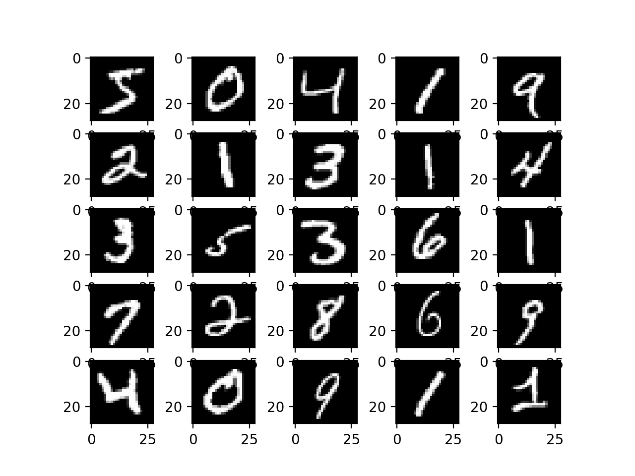
A popular image classification task is the MNIST handwritten digit classification. It involves tens of thousands of handwritten digits that must be classified as a number between 0 and 9.
The tf.keras API provides a convenient function to download and load this dataset directly.
The example below loads the dataset and plots the first few images.
1
2
3
4
5
6
7
8
9
10
11
12
13
14
15
16
# example of loading and plotting the mnist dataset
from tensorflow.keras.datasets.mnist import load_data
Running the example loads the MNIST dataset, then summarizes the default train and test datasets.
1
2
Train: X=(60000, 28, 28), y=(60000,)
Test: X=(10000, 28, 28), y=(10000,)
A plot is then created showing a grid of examples of handwritten images in the training dataset.
Plot of Handwritten Digits From the MNIST dataset
We can train a CNN model to classify the images in the MNIST dataset.
Note that the images are arrays of grayscale pixel data; therefore, we must add a channel dimension to the data before we can use the images as input to the model. The reason is that CNN models expect images in a channels-last format; that is, each example to the network has the dimensions [rows, columns, channels], where channels represent the color channels of the image data.
It is also a good idea to scale the pixel values from the default range of 0-255 to 0-1 when training a CNN. For more on scaling pixel values, see the tutorial:
Running the example first reports the shape of the dataset then fits the model and evaluates it on the test dataset. Finally, a prediction is made for a single image.
Note: Your results may vary given the stochastic nature of the algorithm or evaluation procedure, or differences in numerical precision. Consider running the example a few times and compare the average outcome.
What results did you get? Can you change the model to do better?
Post your findings in the comments below.
First, the shape of each image is reported along with the number of classes; we can see that each image is 28×28 pixels, and there are 10 classes, as we expected.
In this case, we can see that the model achieved a classification accuracy of about 98% on the test dataset. We can then see that the model predicted class 5 for the first image in the training set.
1
2
3
(28, 28, 1) 10
Accuracy: 0.987
Predicted: class=5
3.3 Develop Recurrent Neural Network Models
Recurrent Neural Networks, or RNNs for short, are designed to operate upon sequences of data.
They have proven to be very effective for natural language processing problems where sequences of text are provided as input to the model. RNNs have also seen some modest success in time series forecasting and speech recognition.
The most popular type of RNN is the Long Short-Term Memory network or LSTM for short. LSTMs can be used in a model to accept a sequence of input data and make a prediction, such as assign a class label or predict a numerical value like the next value or values in the sequence.
You will use the car sales dataset to demonstrate an LSTM RNN for univariate time series forecasting.
This problem involves predicting the number of car sales per month.
The dataset will be downloaded automatically using Pandas, but you can learn more about it here.
Let’s frame the problem to take a window of the last five months of data to predict the current month’s data.
To achieve this, you define a new function named split_sequence() that will split the input sequence into windows of data appropriate for fitting a supervised learning model, like an LSTM.
For example, if the sequence was:
1
1, 2, 3, 4, 5, 6, 7, 8, 9, 10
Then the samples for training the model would look like:
1
2
3
4
5
Input Output
1, 2, 3, 4, 5 6
2, 3, 4, 5, 6 7
3, 4, 5, 6, 7 8
...
Use the last 12 months of data as the test dataset.
LSTMs expect each sample in the dataset to have two dimensions; the first is the number of time steps (in this case, it is 5), and the second is the number of observations per time step (in this case, it is 1).
Because it is a regression-type problem, we will use a linear activation function (no activation function) in the output layer and optimize the mean squared error loss function. We will also evaluate the model using the mean absolute error (MAE) metric.
The complete example of fitting and evaluating an LSTM for a univariate time series forecasting problem is listed below.
Running the example first reports the shape of the dataset then fits the model and evaluates it on the test dataset. Finally, a prediction is made for a single example.
Note: Your results may vary given the stochastic nature of the algorithm or evaluation procedure, or differences in numerical precision. Consider running the example a few times and compare the average outcome.
What results did you get? Can you change the model to do better?
Post your findings in the comments below.
First, the shape of the train and test datasets is displayed, confirming that the last 12 examples are used for model evaluation.
In this case, the model achieved an MAE of about 2,800 and predicted the next value in the sequence from the test set as 13,199, where the expected value is 14,577 (pretty close).
1
2
3
(91, 5, 1) (12, 5, 1) (91,) (12,)
MSE: 12755421.000, RMSE: 3571.473, MAE: 2856.084
Predicted: 13199.325
Note: it is good practice to scale and make the series stationary data prior to fitting the model. I recommend this as an extension to achieve better performance. For more on preparing time series data for modeling, see the tutorial:
In this section, you will discover how to use some of the slightly more advanced model features, such as reviewing learning curves and saving models for later use.
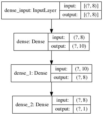
4.1 How to Visualize a Deep Learning Model
The architecture of deep learning models can quickly become large and complex.
As such, it is important to have a clear idea of the connections and data flow in your model. This is especially important if you are using the functional API to ensure you have indeed connected the layers of the model in the way you intended.
There are two tools you can use to visualize your model: a text description and a plot.
Model Text Description
A text description of your model can be displayed by calling the summary() function on your model.
The example below defines a small model with three layers and then summarizes the structure.
Running the example creates a plot of the model showing a box for each layer with shape information and arrows that connect the layers, showing the flow of data through the network.
Plot of Neural Network Architecture
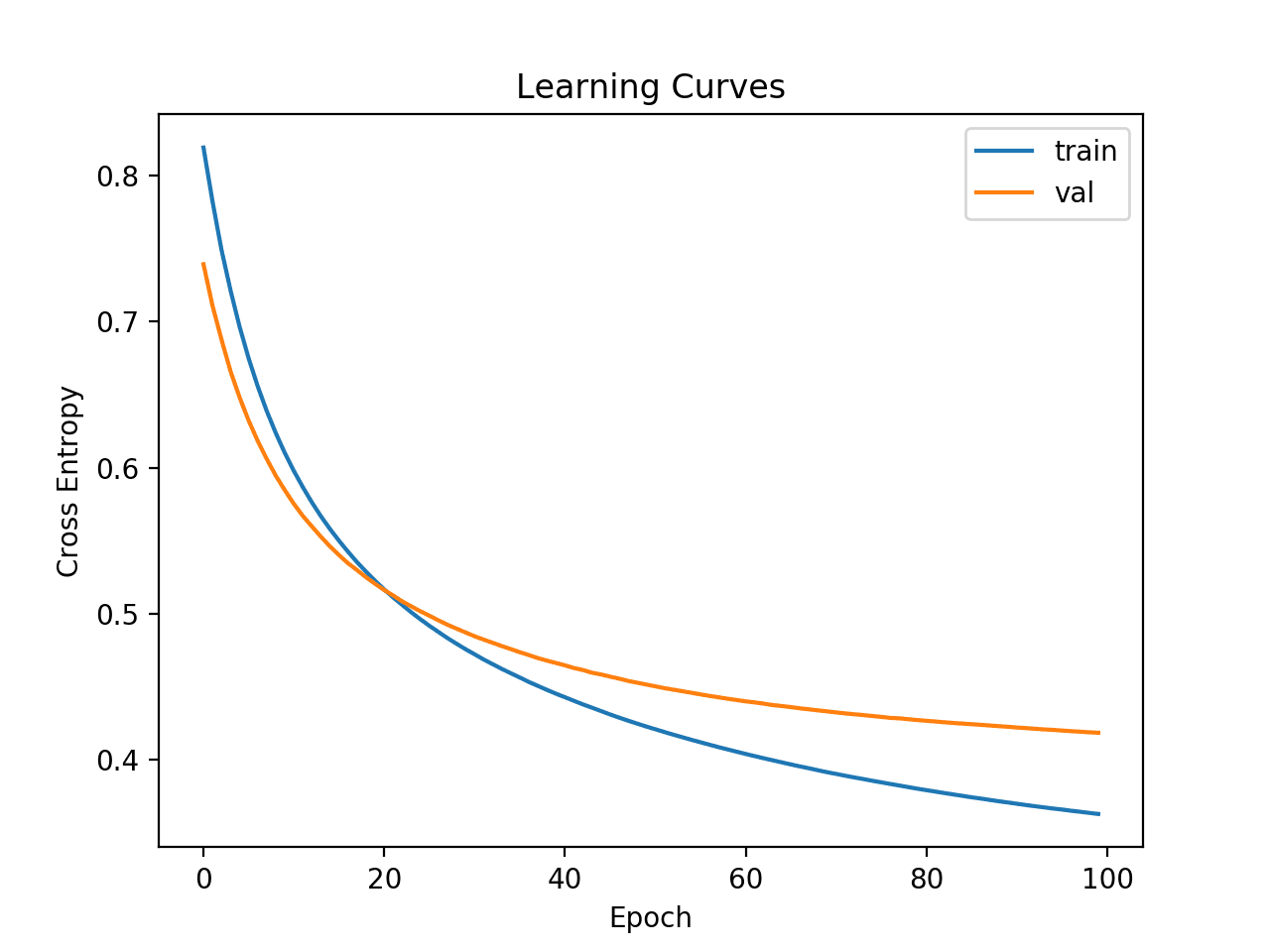
4.2 How to Plot Model Learning Curves
Learning curves are a plot of neural network model performance over time, such as those calculated at the end of each training epoch.
Plots of learning curves provide insight into the learning dynamics of the model, such as whether the model is learning well, underfitting the training dataset, or overfitting the training dataset.
For a gentle introduction to learning curves and how to use them to diagnose the learning dynamics of models, see the tutorial:
You can easily create learning curves for your deep learning models.
First, you must update your call to the fit function to include a reference to a validation dataset. This is a portion of the training set not used to fit the model and is instead used to evaluate the performance of the model during training.
You can split the data manually and specify the validation_data argument, or you can use the validation_split argument and specify a percentage split of the training dataset and let the API perform the split for you. The latter is simpler for now.
The fit function will return a history object that contains a trace of performance metrics recorded at the end of each training epoch. This includes the chosen loss function and each configured metric, such as accuracy, and each loss and metric is calculated for the training and validation datasets.
A learning curve is a plot of the loss on the training dataset and the validation dataset. We can create this plot from the history object using the Matplotlib library.
The example below fits a small neural network on a synthetic binary classification problem. A validation split of 30% is used to evaluate the model during training, and the cross-entropy loss on the train and validation datasets are then graphed using a line plot.
Running the example fits the model on the dataset. At the end of the run, the history object is returned and used as the basis for creating the line plot.
The cross-entropy loss for the training dataset is accessed via the ‘loss‘ key, and the loss on the validation dataset is accessed via the ‘val_loss‘ key on the history attribute of the history object.
Learning Curves of Cross-Entropy Loss for a Deep Learning Model
4.3 How to Save and Load Your Model
Training and evaluating models is great, but we may want to use a model later without retraining it each time.
This can be achieved by saving the model to a file, loading it later, and using it to make predictions.
This can be achieved using the save() function on the model to save the model. It can be loaded later using the load_model() function.
The model is saved in H5 format, an efficient array storage format. As such, you must ensure that the h5py library is installed on your workstation. This can be achieved using pip, for example:
1
pip install h5py
The example below fits a simple model on a synthetic binary classification problem and then saves the model file.
Running the example loads the image from the file, then uses it to make a prediction on a new row of data and prints the result.
1
Predicted: 0.831
5. How to Get Better Model Performance
In this section, you will discover some of the techniques that you can use to improve the performance of your deep learning models.
A big part of improving deep learning performance involves avoiding overfitting by slowing down the learning process or stopping the learning process at the right time.
5.1 How to Reduce Overfitting with Dropout
Dropout is a clever regularization method that reduces the overfitting of the training dataset and makes the model more robust.
This is achieved during training, where some number of layer outputs are randomly ignored or “dropped out.” This has the effect of making the layer look like—and be treated like—a layer with a different number of nodes and connectivity to the prior layer.
Dropout has the effect of making the training process noisy, forcing nodes within a layer to take on more or less responsibility for the inputs probabilistically.
You can add dropout to your models as a new layer prior to the layer that you want to have input connections dropped out.
This involves adding a layer called Dropout() that takes an argument specifying the probability that each output from the previous will drop, e.g., 0.4 means 40% percent of inputs will be dropped each update to the model.
You can add Dropout layers in MLP, CNN, and RNN models, although there are also specialized versions of dropout for use with CNN and RNN models that you might also want to explore.
The example below fits a small neural network model on a synthetic binary classification problem.
A dropout layer with 50% dropout is inserted between the first hidden layer and the output layer.
5.2 How to Accelerate Training with Batch Normalization
The scale and distribution of inputs to a layer can greatly impact how easy or quickly that layer can be trained.
This is generally why it is a good idea to scale input data prior to modeling it with a neural network model.
Batch normalization is a technique for training very deep neural networks that standardizes the inputs to a layer for each mini-batch. This has the effect of stabilizing the learning process and dramatically reducing the number of training epochs required to train deep networks.
For more on how batch normalization works, see this tutorial:
You can use batch normalization in your network by adding a batch normalization layer prior to the layer that you wish to have standardized inputs. You can use batch normalization with MLP, CNN, and RNN models.
The example below defines a small MLP network for a binary classification prediction problem with a batch normalization layer between the first hidden layer and the output layer.
1
2
3
4
5
6
7
8
9
10
11
12
13
14
15
16
17
18
19
# example of using batch normalization
from sklearn.datasets import make_classification
from tensorflow.keras import Sequential
from tensorflow.keras.layers import Dense
from tensorflow.keras.layers import BatchNormalization
5.3 How to Halt Training at the Right Time with Early Stopping
Neural networks are challenging to train.
Too little training and the model is underfit; too much training and the model overfits the training dataset. Both cases result in a model that is less effective than it could be.
One approach to solving this problem is to use early stopping. This involves monitoring the loss on the training dataset and a validation dataset (a subset of the training set not used to fit the model). As soon as loss for the validation set starts to show signs of overfitting, the training process can be stopped.
Early stopping can be used with your model by first ensuring that you have a validation dataset. You can define the validation dataset manually via the validation_data argument to the fit() function, or you can use the validation_split and specify the amount of the training dataset to hold back for validation.
You can then define an EarlyStopping and instruct it on which performance measure to monitor, such as ‘val_loss‘ for loss on the validation dataset and the number of epochs to observe overfitting before taking action, e.g., 5.
This configured EarlyStopping callback can then be provided to the fit() function via the “callbacks” argument that takes a list of callbacks.
This allows you to set the number of epochs to a large number and be confident that training will end as soon as the model starts overfitting. You might also want to create a learning curve to discover more insights into the learning dynamics of the run and when training was halted.
The example below demonstrates a small neural network on a synthetic binary classification problem that uses early stopping to halt training as soon as the model starts overfitting (after about 50 epochs).
1
2
3
4
5
6
7
8
9
10
11
12
13
14
15
16
17
18
19
# example of using early stopping
from sklearn.datasets import make_classification
from tensorflow.keras import Sequential
from tensorflow.keras.layers import Dense
from tensorflow.keras.callbacks import EarlyStopping
In case of the MLP for Regression example, by the first hidden layer with 10 nodes, if I change the activation function from ‘relu’ to ‘sigmoid’ I always get much better result: Following couple of tries with that change:
To add on the discussion of ‘Relu’ vs ‘Sigmoid’ output function, ‘Relu’ is used after ‘Sigmoid’ has the problem of disappearing gradient for deep structure network, like 30-100 layers. The particular example used here is actually more a ‘shallow’ network relative to the ‘deep’ one more people are used in real project these days. So, it’s not surprised that a ‘sigmoid’ function is fine or even better.
Awesome stuff. It has very good information on TensorFlow 2. Best guide to developing deep learning models for Business intelligence .Thanks for sharing!
Also, the end of epoch loss/accuracy is an average over the batches, it is better to call evaluate() at the end of the run to get a true estimate of model performance on a hold out dataset.
thanks Jason brownlee!
i am following your tutorial since i start my machine/deep learning journey, it really help me alot. Since deep learning models are becoming bigger which require multi-GPU support. It will be great if you write a tutorial on tf.keras for multi-GPU preferably some GAN model like CycleGAN or MUNIT. Thank
Hi Israr and Jason, yes I second that, it a tutorial for multi gpu using Keras would be awesome. That said, I am reading about issued of multi GPU not working with a number of tensorflow backend versions. Thanks, Mark
Thanks for another great post!
In the functional model API section you mention that this allows for multiple input paths. My question is related to that. The output of my MLP model will be reshaped and 2d convolved with an image (another data input midstream to the network). How do I keep this result as a part of the overall model for further processing? (model.add(intermediate_result)?)
Thanks.
This blog was written so well, it filled me up with emotions!
I am now doing the monthly donation. And I would suggest for everyone to give back to this awesome blog to keep it up and running!
Thank you Jason for this fantastic initiative, you are literally creating jobs!
Great tutorial ! It is a good summary of different MLP, CNN and RNN models (including the datasets cases approached by simple few lines codes). Congratulations !.
1.) Here are my results, at the time being I have only worked with Ionosphere and Iris data cases (I will continue the next ones) but, I share the first two:
1.1) in the fist Ionosphere study Case (MLP model for Binary Classification), I apply some differences (complementing your codes) such as:
80% training data, 10% validation data (that I included in model.fit data) and 10% test data (unseen for accuracy evaluation). Plus I add batchnormalization and dropout (0.5) layers to each of any dense layer (for regularization purposes) and I use 34 units and 8 units for the 2 hidden layers respectively.
I got 97.2% (a little be better of yours 94.% accuracy for unseen test) and 97.3% class good for the example given
1.2) in the second Iris study Case (MLP Multiclassification), I apply some differences (complementing your codes) such as:
80% training data, 10% validation data (I include in model.fit data) and 10% test data (unseen for accuracy evaluation). Plus I add batchnormalization and dropout (0.5) layers to each of any dense layer (for regularization purposes) and I use 64 units, 32 units and 8 units for the now 3 hidden layers respectively.
I got 100.% (a little be better of yours 98.% accuracy for unseen test) and 99.9% class Iris-setosa for the example given
2.) Here are my persistent doubts, in case you can help me:
2.1) if applyng tf.keras new wrapper over tf. 2.x version it is only impact on change the libraries importation such as for example replacing this Keras one example:
from keras.utils import plot_model
for a new one using the tf.keras wrappers
from tensorflow.keras.utils import plot_model
it is highly recommended to apply tf.keras directly due to better guarantee of maintenance by Google/tensorflow team. Do you agree?
2.2) do you expect any efficiency improvement (e.g. on execution time) using tf.keras vs keras ? I apply it but I do not see any change at all. Do you agree?
2.3) I see you have changed loss parameter in Multiclassification (e.g. Iris study case) from previous tutorials of your from categorical_crossentropy to the new one sparse_categorical_crossentroypy. I think it is better the second one. Do you agree?
thank you very much for make these awesome tutorials for us!!
I will continue with the rest of study cases under this tutorial !
I spent some time implementing different models for MNIST Images Digits Multiclass.
Here I share my main comments:
the 10,000 Test Image I split between 5,000 for Validation (besides training images) and another 5,000 for test (unseeing images for model.evaluate() ), so I think it is more Objetive.
1.) Replicating your same model architecture I got 98.3% Accuracy and, if I replace your 32 filters of your first Conv2D layer for “784” filters I got 98.2%, but the 2 minutes CPU time goes to 45 minutes.
2.) I define a new model with “4 blocks” of increasing number of filters [16,32,64,128] of conv2D`s plus batchnormalization+MaxPoool2D+ Dropout layers as regularizers. But I got I worst result (97.2% and 97.4% if I replace the batch size from 128 for 32).
3.) I apply “Data Augmentation” to your model (with soft images distortion due to poor 28×28 resolution), but I got 96.7%, 97.3% and 97.9% respectively for witdth_shift_range adn similiar height_shiftrange_ arguments values of 0.1, 0.05 and 0.01.
3.1) But also Applying “reTrain” (from 10 epochs to 20 epochs and even 40 epochs9 where I get 98.2% Accuracy, very close to your model.
I noticed that tensorflow.keras… apply the unique method of “model.fit() “even with ‘ImageDataGenerator’.So “model.fit_genetator()” of keras for imaging iterator is going to be deprecated !
4.) I apply ‘transfer learning’, using VGG16.
But first I have to expand each 28×28 pixels image to 32×32 (VGG16 requirement), filling with zeros the rest of rows and columns of image. I also expand from 1 channel Black/White to 3 channel (VGG16 requirement), stacking the same image 3 times ( np.stack() for the new axis) and,
4.1) I got a poor result of 95.2% accuracy for frozen the whole VGG16 (5 blocks) and using only head dense layer as trainable.
4.2) I reTraining several more epochs + 10 + 10 etc. I got moderate accuracy results such as 96.2% and 96.7%
4.3) I decided to “defrost” (be trainable) also the last block (5º) of VGG16 and I got for 10 epoch 97.2% but I went from 2 minutes CPU time to 45 minutes and also from 52 K weights to 7.1 M trainable
4.3) I decided to “defrost” also the penultimate block number 4th (so 4 and 5 blocks are trainable ) and I went from 45minutes to 85 minutes of CPU and from 7.1 M parameters to 13. M trainable parameters. But I got 98.4 % Accuracy
4.4) Finally I “reTrain” the VGG16 (defrosting 4 and 5th block) and I got for 20 more epochs and 20 more 99.4% and 99.4% also replacing ‘Adam’ optimizer by more soft “SGD” for fine tuning.
At the cost of increasing cpu time goes from 45 minutes to 85 minutes.
My conclusions are:
a) your simple model is very efficient, and robust (without implementing any complexity such as data_augmentation)
b) I can beat yours result I get the best one 99.4%, at the cost fo implementing VGG16 transfer Learning, besides defrosting 4th and 5 blocks of VGG16. At the cost of more complexity and more CPU time.
c) These models are sensitives to retrain from the 10 initial epochs up to 40 where the system does nor learn anymore.
You showed how to predict for one instance of data, but how to do the same for all the test dataset? Instead of passing yhat = model.predict([row]) what should we do to get all the predictions from the test dataset?
Hi Jason, thank you too much for the helpful topic.
I have a problem that I need your help on it.
Due to the suggestion from keras.io and from your topic, I turned to use “tf.keras” instead of “keras” to build my Deep NNs model. I am trying to define a custom loss function for my model.
Firstly, I took a look at how “tf.keras” and “keras” define (by codes) their loss function so that I could follow for my custom loss fn. I took the available MeanSquaredError() for the observation, and I found that they don’t seem to give identical results. Particularly,
My first case ===========================================================
Well, the former gives the “dtype=int32” and the later gives “dtype=float32” although they were run with the same input data.
So, what could be the explanations for the difference?
I believe, when the model is trained, the loss values are unlikely to be integer, so is it a problem if I use the “tf.keras.losses.MeanSquaredError()” for my model?
Lastly, is there any problem of using some loss fns from keras.losses for the model.compile() if the model is built by tf.keras.Sequential()?
I have been trying to implement this for a few days and I have not been successful.
I am getting the errors: ERROR:
root:Internal Python error in the inspect module.
Below is the traceback from this internal error.
Traceback (most recent call last):
File “C:\ProgramData\Anaconda3\lib\site-packages\IPython\core\interactiveshell.py”, line 3331, in run_code
exec(code_obj, self.user_global_ns, self.user_ns)
File “”, line 1, in
model = tf.keras.Sequential()
AttributeError: module ‘tensorflow’ has no attribute ‘keras’
WARNING:tensorflow:From D:\Anaconda3\lib\site-packages\tensorflow\python\ops\resource_variable_ops.py:435: colocate_with (from tensorflow.python.framework.ops) is deprecated and will be removed in a future version.
Instructions for updating:
Colocations handled automatically by placer.
WARNING:tensorflow:From D:\Anaconda3\lib\site-packages\tensorflow\python\ops\math_ops.py:3066: to_int32 (from tensorflow.python.ops.math_ops) is deprecated and will be removed in a future version.
Instructions for updating:
Use tf.cast instead.
Test Accuracy: 0.914
Traceback (most recent call last):
File “D:\tflowdata\untitled3.py”, line 44, in
yhat = model.predict([row])
File “D:\Anaconda3\lib\site-packages\tensorflow\python\keras\engine\training.py”, line 1096, in predict
x, check_steps=True, steps_name=’steps’, steps=steps)
I cut and paste the example and got this error:
How did I get it wrong?
import tensorflow
print(tensorflow.__version__)# example of a model defined with the sequential api
from tensorflow.keras import Sequential
from tensorflow.keras.layers import Dense
# define the model
model = Sequential()
model.add(Dense(100, input_shape=(8,0)))
model.add(Dense(80))
model.add(Dense(30))
model.add(Dense(10))
model.add(Dense(5))
model.add(Dense(1))
2.1.0
—————————————————————————
InternalError Traceback (most recent call last)
in
6 # define the model
7 model = Sequential()
—-> 8 model.add(Dense(100, input_shape=(8,0)))
9 model.add(Dense(80))
10 model.add(Dense(30))
~\Anaconda3\lib\site-packages\tensorflow_core\python\keras\engine\sequential.py in add(self, layer)
183 # and create the node connecting the current layer
184 # to the input layer we just created.
–> 185 layer(x)
186 set_inputs = True
187
~\Anaconda3\lib\site-packages\tensorflow_core\python\keras\engine\base_layer.py in __call__(self, inputs, *args, **kwargs)
746 # Build layer if applicable (if the build method has been
747 # overridden).
–> 748 self._maybe_build(inputs)
749 cast_inputs = self._maybe_cast_inputs(inputs)
750
~\Anaconda3\lib\site-packages\tensorflow_core\python\keras\engine\base_layer.py in _maybe_build(self, inputs)
2114 # operations.
2115 with tf_utils.maybe_init_scope(self):
-> 2116 self.build(input_shapes)
2117 # We must set self.built since user defined build functions are not
2118 # constrained to set self.built.
I did find the problem:
I had been successfully using TensorFlow-GPU 1 and Keras.
When I upgraded to 2, this same code failed.
It was because my NVIDIA CUDA drivers needed to be updated in order to support TF 2.
Sorry for the question, but maybe it will help someone else.
Hi Jason, in your example for regression for boston house price prediction, the mse is about 60. Is it ok for a prediction to have mean square error with a high value?Sorry for asking.
With MNIST CNN model, I get the good “fit” to the data. When I run:
# make a prediction
image = x_train[0]
yhat = model.predict([[image]])
print(‘Predicted: class=%d’ % argmax(yhat))
at the end of the model, “yhat = model.predict([[image]])” I get a Value Error:
ValueError Traceback (most recent call last)
in
41 #yhat = model.predict([[image]]) all these gave errors
42 #yhat = model.predict([image])
—> 43 yhat = model.predict(image)
44 print(‘Predicted: class={0}’.format(argmax(yhat)))
45 #should get for output
~\Anaconda3\lib\site-packages\tensorflow\python\keras\engine\training.py in _method_wrapper(self, *args, **kwargs)
86 raise ValueError(‘{} is not supported in multi-worker mode.’.format(
87 method.__name__))
—> 88 return method(self, *args, **kwargs)
89
90 return tf_decorator.make_decorator(
~\Anaconda3\lib\site-packages\tensorflow\python\keras\engine\training.py in predict(self, x, batch_size, verbose, steps, callbacks, max_queue_size, workers, use_multiprocessing)
1266 for step in data_handler.steps():
1267 callbacks.on_predict_batch_begin(step)
-> 1268 tmp_batch_outputs = predict_function(iterator)
1269 # Catch OutOfRangeError for Datasets of unknown size.
1270 # This blocks until the batch has finished executing.
~\Anaconda3\lib\site-packages\tensorflow\python\eager\def_function.py in __call__(self, *args, **kwds)
578 xla_context.Exit()
579 else:
–> 580 result = self._call(*args, **kwds)
581
582 if tracing_count == self._get_tracing_count():
~\Anaconda3\lib\site-packages\tensorflow\python\eager\def_function.py in _call(self, *args, **kwds)
625 # This is the first call of __call__, so we have to initialize.
626 initializers = []
–> 627 self._initialize(args, kwds, add_initializers_to=initializers)
628 finally:
629 # At this point we know that the initialization is complete (or less
~\Anaconda3\lib\site-packages\tensorflow\python\eager\function.py in _create_graph_function(self, args, kwargs, override_flat_arg_shapes)
2665 arg_names=arg_names,
2666 override_flat_arg_shapes=override_flat_arg_shapes,
-> 2667 capture_by_value=self._capture_by_value),
2668 self._function_attributes,
2669 # Tell the ConcreteFunction to clean up its graph once it goes out of
~\Anaconda3\lib\site-packages\tensorflow\python\eager\def_function.py in wrapped_fn(*args, **kwds)
439 # __wrapped__ allows AutoGraph to swap in a converted function. We give
440 # the function a weak reference to itself to avoid a reference cycle.
–> 441 return weak_wrapped_fn().__wrapped__(*args, **kwds)
442 weak_wrapped_fn = weakref.ref(wrapped_fn)
443
~\Anaconda3\lib\site-packages\tensorflow\python\framework\func_graph.py in wrapper(*args, **kwargs)
966 except Exception as e: # pylint:disable=broad-except
967 if hasattr(e, “ag_error_metadata”):
–> 968 raise e.ag_error_metadata.to_exception(e)
969 else:
970 raise
I am a big fanboy of your tutorial … I get to learn a lot from your tutorial… please accept my gratitude for the same and really thank you for sharing knowledge in best possible way….
One update:
Code for ‘Develop Convolutional Neural Network Models’ has one small bug related to the mismatch of model’s input dimension against providing input’s dimension for prediction in line no: 41:
yhat = model.predict([[image]])
correct line could be :
—————————–
from numpy import array
yhat = model.predict(array([image]))
I have already ran the code and posting this update.
P.S. I could be wrong … in that case please correct me
When model.fit() finishes, the deep model has the weights if the best model found during the epochs?
Or should I use a ModelCheckpoint callback, with save_best_only=True, and after .fit() to load the ‘best’ weights and then .evaluate(X_test, y_test) and in order to get some metrics?
Hey , thanks a lot for creating this kind of tutorial really i want this and i found it i learn a lot from your tutorial , can you please create a web app with ml and django , please i needed
Hi Jason. Thanks for your sharing! I have a question that in the Convolutional Neural Network Model, why you use the training image (x_train[0]) to predict, shouldn’t we use an unseen image?
I figured out the mistake I had made.
I had typed
X_train, y_train,X_test, y_test = train_test_split(X, y, test_size=0.33) instead of X_train, X_test, y_train, y_test = train_test_split(X, y, test_size=0.33)
Great tutorials! I have just initiated learning DL and I only refer your content because it’s so clear! Thanks again.
Hi Jason. I don’t understand this line
#CNN
x_train = x_train.reshape((x_train.shape[0], x_train.shape[1], x_train.shape[2], 1))
Can you please explain what it does? Thank you
In the section for the “MLP for Binary Classification”, the code has this line:
model.compile(optimizer=’adam’, loss=’binary_crossentropy’, metrics=[‘accuracy’])
I tried switching back and forth between metrics=[‘accuracy’] and metrics=[‘binary_accuracy’], and it didn’t seem to make any difference in the quality of the results, so I’m not sure what the difference between the two is intended to be.
model = tf.keras.metrics.Accuracy()
model.update_state(y_true, y_pred)
print(“Accuracy: “, model.result().numpy())
model = tf.keras.metrics.BinaryAccuracy()
model.update_state(y_true, y_pred)
print(“Binary Accuracy: “, model.result().numpy())
#####
Running this code results in the following.
Accuracy: 0.25
Binary Accuracy: 0.75
I don’t understand why this difference in behavior doesn’t manifest in the Binary Classification model from this tutorial. It seems like switching the model’s metrics from ‘accuracy’ to ‘binary_accuracy’ should make a huge difference, as in the above test code, but in fact it makes no discernible difference. There must be something fundamental that I’m misunderstanding.
I have a question about the Dropout regularization in the CNN example with the numbers set. I have tried the same model but I replaced the dropout with an L2 regularization but I got an accuracy of about 0.981 so it was slightly lower than the Dropout accuracy (0.987). So I just wanted to know if there is a way to know which regularization technique might be the most suitable for our training set.
hi Jason, thank you for this tutorial
i have dummy questions
in the codes where is the initialization of weights?
can we use tensorflow to build a model without keras ?!
someone told me that if we don’t mention the initialize of weights, it will take the value of learning rate as an initialize value for all weights of the model and then by training it will be updated ?
How to add log loss metric to mlp_multiclass_classification ? This does not work : model.compile(optimizer=’adam’, loss=’sparse_categorical_crossentropy’, metrics=[‘log_loss’])
How to add r2 metric to mlp_regression ? This does not work : model.compile(optimizer=’adam’, loss=’mse’, metrics=[tfa.metrics.r_square.RSquare()])
For r2, using hand-written r2_square, I get this kind of errors “NotImplementedError: Cannot convert a symbolic Tensor (ExpandDims:0) to a numpy array. This error may indicate that you’re trying to pass a Tensor to a NumPy call, which is not supported” ?!…
And using sklearn.metrics.r2_square, I get “OperatorNotAllowedInGraphError: using a tf.Tensor as a Python bool is not allowed: AutoGraph did convert this function. This might indicate you are trying to use an unsupported feature.”
Yes, just verified. Except I would remove the import statement inside the function. Tensorflow’s Keras not always have all metric functions, especially for those function that might be misleading if applied to small batch (e.g., R^2 and F1).
I’ve tried the first 3 code examples on a clean installed box and each one yields an error similar to “ValueError: Error when checking input: expected dense_input to have shape (13,) but got array with shape (1,)” (which is from the 3rd example). What am I missing here?
Hi,
Thanks for the article it is great to have an overview of Deep Learning and Tensorflow 2 !
Could you explain the difference between trainable and non-trainable params ?
Have a nice day 🙂
Hi Jason, thank you for this tutorial. I notice that you used LabelEncoder() before doing the train/test split, but this is usually regarded as data leakage. Am I understanding correctly?
Wow, this is such a thorough learning guide, Jason. As someone who is fairly new to TensorFlow and deep learning, I!m glad I stumbled upon this tutorial! I appreciate that you’ve also highlighted the distinction between Keras and tf.keras; it helped clear up some things I had found a bit confusing before.
I specifically found the step-by-step approach to installing TensorFlow and tf.keras quite useful. The process looks less daunting now, and I’m looking forward to seeing those version numbers pop up on my screen after successful installation.
And thanks for emphasizing that this is a practical guide and I don’t necessarily need to grasp everything at once, that takes a good chunk of learning anxiety away. I look forward to diving into the codes and learning through doing, which I agree, in my experience, is one of the most effective ways to learn programming.
I’m particularly excited about eventually understanding how to develop Multilayer Perceptron Models, Convolutional Neural Network Models, and Recurrent Neural Network Models. And learning about ways to improve model performance piques my interest too!
Just a question, as I immerse myself in this, I wonder if there are any common pitfalls or misconceptions I should be aware of when starting out with TensorFlow and deep learning in general?
Again, excellent piece, Jason! I’m all set to embark on this deep learning journey with your guide as my compass. Can’t wait to deepen my understanding even more and apply these key learnings to real-world problems. Thanks for sharing your expertise and for making deep learning more accessible for beginners like me!
Hi AI…Thank you for your feedback and support! One pitfall would be applying the “latest and greatest” AI tool or technique without consideration of time-tested techniques and models first.
The following resource is a great starting point to begin your machine learning journey with our content:

")

")
")


Hi
Thanks for this awesome blog post.
In case of the MLP for Regression example, by the first hidden layer with 10 nodes, if I change the activation function from ‘relu’ to ‘sigmoid’ I always get much better result: Following couple of tries with that change:
MSE: 1078.271, RMSE: 32.837
Predicted: 154.961
MSE: 1306.771, RMSE: 36.149
Predicted: 153.267
MSE: 2511.747, RMSE: 50.117
Predicted: 142.649
Do you know why?
Sorry I meant vice versa, that’s ‘sigmoid’ to ‘relu’.
Agreed.
I found the same and updated the example accordingly.
Thanks Markus!
You’re welcome.
Nice finding, I’ll explore and update the post.
The reason. My guess is the data needs to be transformed prior to scaling.
Hi
Thanks.
Could you please elaborate your answer a bit as I didn’t understand it? That model doesn’t have any scaling like the CNN example.
Yes, I believe that the model would perform better with sigmoid activations if the data was scaled (normalized) prior to fitting the model.
The relu is more robust and is in less need of normalized inputs.
Jason, This is a great tutorial on TF 2.0 !
To add on the discussion of ‘Relu’ vs ‘Sigmoid’ output function, ‘Relu’ is used after ‘Sigmoid’ has the problem of disappearing gradient for deep structure network, like 30-100 layers. The particular example used here is actually more a ‘shallow’ network relative to the ‘deep’ one more people are used in real project these days. So, it’s not surprised that a ‘sigmoid’ function is fine or even better.
Thanks!
Yes, this gives an example:
https://machinelearningmastery.com/how-to-fix-vanishing-gradients-using-the-rectified-linear-activation-function/
# mlp for regression
Why use y = LabelEncoder().fit_transform(y)? It’s not necessary, and the prediction of yhat() is too large than y which max is 50.0,
You’re right, looks like a bug!
Thanks Todd.
Updated.
Little bug in last example:
from:
from keras.callbacks import EarlyStopping
to:
from tensorflow.keras.callbacks import EarlyStopping
Thanks, fixed!
Is it necessary yo set a seed before fitting the model?
No.
well explained and liked very much . I request you to please write one blog using below steps?
1) tf.keras.layers.GRUCell()
2) tf.keras.layers.LSTMCell()
3) tf.nn.RNNCellDropoutWrapper()
4) tf.keras.layers.RNN()
Great suggestions!
Awesome stuff. It has very good information on TensorFlow 2. Best guide to developing deep learning models for Business intelligence .Thanks for sharing!
Thanks!
Nice guide! Thanks a lot!
I have a question related to the MLP Binary Classification problem.
During the evaluation process, i’ve changed the verbose argument to 2, and got this:
116/1 – 0s – loss: 0.1011 – accuracy: 0.9483
I’ve added a print command to show the test loss line:
print(‘Test loss: %.3f’ % loss)
print(‘Test Accuracy: %.3f’ % acc)
And i’m getting this result:
Loss Test: 0.169
Test Accuracy: 0.948
Why is it different from the reported by the evaluate function?
You have clipped precision at 3 decimal places.
Also, the end of epoch loss/accuracy is an average over the batches, it is better to call evaluate() at the end of the run to get a true estimate of model performance on a hold out dataset.
Thank you so much for the blog, provides lot of information to learners
Please help with more information on forecasting using RNN
You’re welcome!
See the tutorials here:
https://machinelearningmastery.com/start-here/#deep_learning_time_series
Hi Jason,
in the CNN example, wouldn’t it be MaxPool2D instead of MaxPooling2D?
I believe you’re correct:
https://www.tensorflow.org/api_docs/python/tf/keras/layers/MaxPool2D
thanks Jason brownlee!
i am following your tutorial since i start my machine/deep learning journey, it really help me alot. Since deep learning models are becoming bigger which require multi-GPU support. It will be great if you write a tutorial on tf.keras for multi-GPU preferably some GAN model like CycleGAN or MUNIT. Thank
Thanks for the suggestion!
Hi Israr and Jason, yes I second that, it a tutorial for multi gpu using Keras would be awesome. That said, I am reading about issued of multi GPU not working with a number of tensorflow backend versions. Thanks, Mark
Thanks.
Thanks for another great post!
In the functional model API section you mention that this allows for multiple input paths. My question is related to that. The output of my MLP model will be reshaped and 2d convolved with an image (another data input midstream to the network). How do I keep this result as a part of the overall model for further processing? (model.add(intermediate_result)?)
Thanks.
Yes, you could have one output for each element you require, e.g. each layer that produces an output you want would be an “output” layer.
See this:
https://machinelearningmastery.com/keras-functional-api-deep-learning/
never mind, I figured it out, the functional API does make it easy!
Well done!
This blog was written so well, it filled me up with emotions!
I am now doing the monthly donation. And I would suggest for everyone to give back to this awesome blog to keep it up and running!
Thank you Jason for this fantastic initiative, you are literally creating jobs!
Thanks!!!
Hi
For the input_shape parameter of a a Dense layer it seems that one can pass over a list instead of a tuple. That’s
model.add(Dense(10, input_shape=[8]))
Instead of:
model.add(Dense(10, input_shape=(8,)))
My questions are:
Is that the same?
Why is that so that both works?
Probably it’s even possible for any layer type that has input_shape parameter (which I’ve not tested).
Thanks
I think I figured it out by myself, BUT please correct me if I’m wrong. It’s happening here:
https://github.com/keras-team/keras/blob/master/keras/engine/base_layer.py#L163
So no matter if you pass over a list or a tuple object, the return value of:
tuple(kwargs[‘input_shape’])
will be always the same as a tuple object because:
>>> tuple((2,))
(2,)
>>> tuple([2])
(2,)
Am I right?
Thanks.
Identical.
Hi Jason
Thanks for your reply.
What do you mean with identical? Sorry my English is a bit poor.
Equilivient. They do the same thing.
Hi Jason,
In Ionosphere data code block line 32, should it be
yhat = model.predict(([row],)) instead of yhat = model.predict([row])?
Just to match the input_shape, which is required to be a one-element tuple?
The model expects 2d input: rows,cols or samples,features.
Hi Jason:
Great tutorial ! It is a good summary of different MLP, CNN and RNN models (including the datasets cases approached by simple few lines codes). Congratulations !.
1.) Here are my results, at the time being I have only worked with Ionosphere and Iris data cases (I will continue the next ones) but, I share the first two:
1.1) in the fist Ionosphere study Case (MLP model for Binary Classification), I apply some differences (complementing your codes) such as:
80% training data, 10% validation data (that I included in model.fit data) and 10% test data (unseen for accuracy evaluation). Plus I add batchnormalization and dropout (0.5) layers to each of any dense layer (for regularization purposes) and I use 34 units and 8 units for the 2 hidden layers respectively.
I got 97.2% (a little be better of yours 94.% accuracy for unseen test) and 97.3% class good for the example given
1.2) in the second Iris study Case (MLP Multiclassification), I apply some differences (complementing your codes) such as:
80% training data, 10% validation data (I include in model.fit data) and 10% test data (unseen for accuracy evaluation). Plus I add batchnormalization and dropout (0.5) layers to each of any dense layer (for regularization purposes) and I use 64 units, 32 units and 8 units for the now 3 hidden layers respectively.
I got 100.% (a little be better of yours 98.% accuracy for unseen test) and 99.9% class Iris-setosa for the example given
2.) Here are my persistent doubts, in case you can help me:
2.1) if applyng tf.keras new wrapper over tf. 2.x version it is only impact on change the libraries importation such as for example replacing this Keras one example:
from keras.utils import plot_model
for a new one using the tf.keras wrappers
from tensorflow.keras.utils import plot_model
it is highly recommended to apply tf.keras directly due to better guarantee of maintenance by Google/tensorflow team. Do you agree?
2.2) do you expect any efficiency improvement (e.g. on execution time) using tf.keras vs keras ? I apply it but I do not see any change at all. Do you agree?
2.3) I see you have changed loss parameter in Multiclassification (e.g. Iris study case) from previous tutorials of your from categorical_crossentropy to the new one sparse_categorical_crossentroypy. I think it is better the second one. Do you agree?
thank you very much for make these awesome tutorials for us!!
I will continue with the rest of study cases under this tutorial !
regards
JG
Nice work, but the test/val sets are very small. I guess we should be using repeated 10 fold cross-validation.
Yes, we should cut over to tf.keras soon:
https://machinelearningmastery.com/faq/single-faq/what-is-the-difference-between-keras-and-tf-keras
Not sure about efficiency differences. No.
They do the same thing, I used the sparse loss so I didn’t have to one hot encode.
Thanks for your valuable suggestions !
I’m hooked on your tutorials !
Thanks!
Hi Jason,
I spent some time implementing different models for MNIST Images Digits Multiclass.
Here I share my main comments:
the 10,000 Test Image I split between 5,000 for Validation (besides training images) and another 5,000 for test (unseeing images for model.evaluate() ), so I think it is more Objetive.
1.) Replicating your same model architecture I got 98.3% Accuracy and, if I replace your 32 filters of your first Conv2D layer for “784” filters I got 98.2%, but the 2 minutes CPU time goes to 45 minutes.
2.) I define a new model with “4 blocks” of increasing number of filters [16,32,64,128] of conv2D`s plus batchnormalization+MaxPoool2D+ Dropout layers as regularizers. But I got I worst result (97.2% and 97.4% if I replace the batch size from 128 for 32).
3.) I apply “Data Augmentation” to your model (with soft images distortion due to poor 28×28 resolution), but I got 96.7%, 97.3% and 97.9% respectively for witdth_shift_range adn similiar height_shiftrange_ arguments values of 0.1, 0.05 and 0.01.
3.1) But also Applying “reTrain” (from 10 epochs to 20 epochs and even 40 epochs9 where I get 98.2% Accuracy, very close to your model.
I noticed that tensorflow.keras… apply the unique method of “model.fit() “even with ‘ImageDataGenerator’.So “model.fit_genetator()” of keras for imaging iterator is going to be deprecated !
4.) I apply ‘transfer learning’, using VGG16.
But first I have to expand each 28×28 pixels image to 32×32 (VGG16 requirement), filling with zeros the rest of rows and columns of image. I also expand from 1 channel Black/White to 3 channel (VGG16 requirement), stacking the same image 3 times ( np.stack() for the new axis) and,
4.1) I got a poor result of 95.2% accuracy for frozen the whole VGG16 (5 blocks) and using only head dense layer as trainable.
4.2) I reTraining several more epochs + 10 + 10 etc. I got moderate accuracy results such as 96.2% and 96.7%
4.3) I decided to “defrost” (be trainable) also the last block (5º) of VGG16 and I got for 10 epoch 97.2% but I went from 2 minutes CPU time to 45 minutes and also from 52 K weights to 7.1 M trainable
4.3) I decided to “defrost” also the penultimate block number 4th (so 4 and 5 blocks are trainable ) and I went from 45minutes to 85 minutes of CPU and from 7.1 M parameters to 13. M trainable parameters. But I got 98.4 % Accuracy
4.4) Finally I “reTrain” the VGG16 (defrosting 4 and 5th block) and I got for 20 more epochs and 20 more 99.4% and 99.4% also replacing ‘Adam’ optimizer by more soft “SGD” for fine tuning.
At the cost of increasing cpu time goes from 45 minutes to 85 minutes.
My conclusions are:
a) your simple model is very efficient, and robust (without implementing any complexity such as data_augmentation)
b) I can beat yours result I get the best one 99.4%, at the cost fo implementing VGG16 transfer Learning, besides defrosting 4th and 5 blocks of VGG16. At the cost of more complexity and more CPU time.
c) These models are sensitives to retrain from the 10 initial epochs up to 40 where the system does nor learn anymore.
regards,
JG
Very cool experiments, great learnings!
Thanks for sharing your findings.
You showed how to predict for one instance of data, but how to do the same for all the test dataset? Instead of passing yhat = model.predict([row]) what should we do to get all the predictions from the test dataset?
Pass in all rows into the predict() function to make a prediction for them.
This will help if you need it:
https://machinelearningmastery.com/how-to-make-classification-and-regression-predictions-for-deep-learning-models-in-keras/
Hi Jason, thank you too much for the helpful topic.
I have a problem that I need your help on it.
Due to the suggestion from keras.io and from your topic, I turned to use “tf.keras” instead of “keras” to build my Deep NNs model. I am trying to define a custom loss function for my model.
Firstly, I took a look at how “tf.keras” and “keras” define (by codes) their loss function so that I could follow for my custom loss fn. I took the available MeanSquaredError() for the observation, and I found that they don’t seem to give identical results. Particularly,
My first case ===========================================================
”
import numpy as np
import tensorflow as tf
y_t = np.array([[1, 2, 3, 4], [8, 9, 1, 5], [7, 8, 7, 13]])
y_p = np.array([[4, 5, 23, 14], [18, 91, 7, 10], [3, 6, 5, 7]])
mse = tf.keras.losses.MeanSquaredError()
loss1 = mse(y_t, y_p)
print(‘—‘)
print(‘tf.keras.losses:’, loss1)
”
The result is:
— tf.keras.losses: tf.Tensor(621, shape=(), dtype=int32) —
My second case =========================================================
”
import numpy as np
import keras
y_t = np.array([[1, 2, 3, 4],[8, 9, 1, 5],[7, 8, 7, 13]])
y_p = np.array([[4, 5, 23, 14],[18, 91, 7, 10],[3, 6, 5, 7]])
mse2 = keras.losses.MeanSquaredError()
loss2 = mse2(y_t, y_p)
print(‘—‘)
print(‘keras.losses:’, loss2)
”
The result is:
— keras.losses: tf.Tensor(621.9167, shape=(), dtype=float32) —
======================================================================
Well, the former gives the “dtype=int32” and the later gives “dtype=float32” although they were run with the same input data.
So, what could be the explanations for the difference?
I believe, when the model is trained, the loss values are unlikely to be integer, so is it a problem if I use the “tf.keras.losses.MeanSquaredError()” for my model?
Lastly, is there any problem of using some loss fns from keras.losses for the model.compile() if the model is built by tf.keras.Sequential()?
I generally recommend sticking with standalone Keras for now:
https://machinelearningmastery.com/faq/single-faq/what-is-the-difference-between-keras-and-tf-keras
I cannot help you debug the conversion, sorry.
Thanks for your reply Jason!
I have been trying to implement this for a few days and I have not been successful.
I am getting the errors: ERROR:
root:Internal Python error in the inspect module.
Below is the traceback from this internal error.
Traceback (most recent call last):
File “C:\ProgramData\Anaconda3\lib\site-packages\IPython\core\interactiveshell.py”, line 3331, in run_code
exec(code_obj, self.user_global_ns, self.user_ns)
File “”, line 1, in
model = tf.keras.Sequential()
AttributeError: module ‘tensorflow’ has no attribute ‘keras’
got it working,
(235, 34) (116, 34) (235,) (116,)
WARNING:tensorflow:From D:\Anaconda3\lib\site-packages\tensorflow\python\ops\resource_variable_ops.py:435: colocate_with (from tensorflow.python.framework.ops) is deprecated and will be removed in a future version.
Instructions for updating:
Colocations handled automatically by placer.
WARNING:tensorflow:From D:\Anaconda3\lib\site-packages\tensorflow\python\ops\math_ops.py:3066: to_int32 (from tensorflow.python.ops.math_ops) is deprecated and will be removed in a future version.
Instructions for updating:
Use tf.cast instead.
Test Accuracy: 0.914
Traceback (most recent call last):
File “D:\tflowdata\untitled3.py”, line 44, in
yhat = model.predict([row])
File “D:\Anaconda3\lib\site-packages\tensorflow\python\keras\engine\training.py”, line 1096, in predict
x, check_steps=True, steps_name=’steps’, steps=steps)
Well done!
I believe you need to upgrade hour version of tensorflow to 2.0 or higher.
I cut and paste the example and got this error:
How did I get it wrong?
import tensorflow
print(tensorflow.__version__)# example of a model defined with the sequential api
from tensorflow.keras import Sequential
from tensorflow.keras.layers import Dense
# define the model
model = Sequential()
model.add(Dense(100, input_shape=(8,0)))
model.add(Dense(80))
model.add(Dense(30))
model.add(Dense(10))
model.add(Dense(5))
model.add(Dense(1))
2.1.0
—————————————————————————
InternalError Traceback (most recent call last)
in
6 # define the model
7 model = Sequential()
—-> 8 model.add(Dense(100, input_shape=(8,0)))
9 model.add(Dense(80))
10 model.add(Dense(30))
~\Anaconda3\lib\site-packages\tensorflow_core\python\training\tracking\base.py in _method_wrapper(self, *args, **kwargs)
455 self._self_setattr_tracking = False # pylint: disable=protected-access
456 try:
–> 457 result = method(self, *args, **kwargs)
458 finally:
459 self._self_setattr_tracking = previous_value # pylint: disable=protected-access
~\Anaconda3\lib\site-packages\tensorflow_core\python\keras\engine\sequential.py in add(self, layer)
183 # and create the node connecting the current layer
184 # to the input layer we just created.
–> 185 layer(x)
186 set_inputs = True
187
~\Anaconda3\lib\site-packages\tensorflow_core\python\keras\engine\base_layer.py in __call__(self, inputs, *args, **kwargs)
746 # Build layer if applicable (if the
buildmethod has been747 # overridden).
–> 748 self._maybe_build(inputs)
749 cast_inputs = self._maybe_cast_inputs(inputs)
750
~\Anaconda3\lib\site-packages\tensorflow_core\python\keras\engine\base_layer.py in _maybe_build(self, inputs)
2114 # operations.
2115 with tf_utils.maybe_init_scope(self):
-> 2116 self.build(input_shapes)
2117 # We must set self.built since user defined build functions are not
2118 # constrained to set self.built.
You have custom code, this may help:
https://machinelearningmastery.com/faq/single-faq/can-you-read-review-or-debug-my-code
I did find the problem:
I had been successfully using TensorFlow-GPU 1 and Keras.
When I upgraded to 2, this same code failed.
It was because my NVIDIA CUDA drivers needed to be updated in order to support TF 2.
Sorry for the question, but maybe it will help someone else.
Well done on fixing your issue!
To predict from a model, I need to set up the test observation row like this:-
row = [[0.00632],[18.00],[2.310],[0],[0.5380],[6.5750],[65.20],[4.0900],[1],[296.0],[15.30],[396.90],[4.98]]
yhat = model.predict(np.array(row).T)
It does not work like in this article:-
row = [0.00632,18.00,2.310,0,0.5380,6.5750,65.20,4.0900,1,296.0,15.30,396.90,4.98]
yhat = model.predict([row])
Why?
Are you sure? Perhaps this will help:
https://machinelearningmastery.com/faq/single-faq/why-does-the-code-in-the-tutorial-not-work-for-me
I guess it is the tensorflow version which is causing the problem. Other code working perfectly (except for predicts).
Great.
Excellent blog. It just covers everything in TF . Thanks again for the great blog.
Thanks!
In the batch normalization part, you make a dense layer, activate it with relu and then perform batch norm.
So, layer -> activation -> batch norm
In models like resnet50, the ordering goes like :
layer -> batch norm -> activation(relu)
Does both of them work the same or does the ordering matter? if it matter then how significant is it?
Would you please answer these….
Great question!
Ordering can matter. Some models prefer to batch norm then relu. Perhaps experiment and discover what works best for your model and dataset.
Hi Jason, in your example for regression for boston house price prediction, the mse is about 60. Is it ok for a prediction to have mean square error with a high value?Sorry for asking.
Good question, see this:
https://machinelearningmastery.com/faq/single-faq/how-to-know-if-a-model-has-good-performance
With MNIST CNN model, I get the good “fit” to the data. When I run:
# make a prediction
image = x_train[0]
yhat = model.predict([[image]])
print(‘Predicted: class=%d’ % argmax(yhat))
at the end of the model, “yhat = model.predict([[image]])” I get a Value Error:
ValueError Traceback (most recent call last)
in
41 #yhat = model.predict([[image]]) all these gave errors
42 #yhat = model.predict([image])
—> 43 yhat = model.predict(image)
44 print(‘Predicted: class={0}’.format(argmax(yhat)))
45 #should get for output
~\Anaconda3\lib\site-packages\tensorflow\python\keras\engine\training.py in _method_wrapper(self, *args, **kwargs)
86 raise ValueError(‘{} is not supported in multi-worker mode.’.format(
87 method.__name__))
—> 88 return method(self, *args, **kwargs)
89
90 return tf_decorator.make_decorator(
~\Anaconda3\lib\site-packages\tensorflow\python\keras\engine\training.py in predict(self, x, batch_size, verbose, steps, callbacks, max_queue_size, workers, use_multiprocessing)
1266 for step in data_handler.steps():
1267 callbacks.on_predict_batch_begin(step)
-> 1268 tmp_batch_outputs = predict_function(iterator)
1269 # Catch OutOfRangeError for Datasets of unknown size.
1270 # This blocks until the batch has finished executing.
~\Anaconda3\lib\site-packages\tensorflow\python\eager\def_function.py in __call__(self, *args, **kwds)
578 xla_context.Exit()
579 else:
–> 580 result = self._call(*args, **kwds)
581
582 if tracing_count == self._get_tracing_count():
~\Anaconda3\lib\site-packages\tensorflow\python\eager\def_function.py in _call(self, *args, **kwds)
625 # This is the first call of __call__, so we have to initialize.
626 initializers = []
–> 627 self._initialize(args, kwds, add_initializers_to=initializers)
628 finally:
629 # At this point we know that the initialization is complete (or less
~\Anaconda3\lib\site-packages\tensorflow\python\eager\def_function.py in _initialize(self, args, kwds, add_initializers_to)
504 self._concrete_stateful_fn = (
505 self._stateful_fn._get_concrete_function_internal_garbage_collected( # pylint: disable=protected-access
–> 506 *args, **kwds))
507
508 def invalid_creator_scope(*unused_args, **unused_kwds):
~\Anaconda3\lib\site-packages\tensorflow\python\eager\function.py in _get_concrete_function_internal_garbage_collected(self, *args, **kwargs)
2444 args, kwargs = None, None
2445 with self._lock:
-> 2446 graph_function, _, _ = self._maybe_define_function(args, kwargs)
2447 return graph_function
2448
~\Anaconda3\lib\site-packages\tensorflow\python\eager\function.py in _maybe_define_function(self, args, kwargs)
2775
2776 self._function_cache.missed.add(call_context_key)
-> 2777 graph_function = self._create_graph_function(args, kwargs)
2778 self._function_cache.primary[cache_key] = graph_function
2779 return graph_function, args, kwargs
~\Anaconda3\lib\site-packages\tensorflow\python\eager\function.py in _create_graph_function(self, args, kwargs, override_flat_arg_shapes)
2665 arg_names=arg_names,
2666 override_flat_arg_shapes=override_flat_arg_shapes,
-> 2667 capture_by_value=self._capture_by_value),
2668 self._function_attributes,
2669 # Tell the ConcreteFunction to clean up its graph once it goes out of
~\Anaconda3\lib\site-packages\tensorflow\python\framework\func_graph.py in func_graph_from_py_func(name, python_func, args, kwargs, signature, func_graph, autograph, autograph_options, add_control_dependencies, arg_names, op_return_value, collections, capture_by_value, override_flat_arg_shapes)
979 _, original_func = tf_decorator.unwrap(python_func)
980
–> 981 func_outputs = python_func(*func_args, **func_kwargs)
982
983 # invariant:
func_outputscontains only Tensors, CompositeTensors,~\Anaconda3\lib\site-packages\tensorflow\python\eager\def_function.py in wrapped_fn(*args, **kwds)
439 # __wrapped__ allows AutoGraph to swap in a converted function. We give
440 # the function a weak reference to itself to avoid a reference cycle.
–> 441 return weak_wrapped_fn().__wrapped__(*args, **kwds)
442 weak_wrapped_fn = weakref.ref(wrapped_fn)
443
~\Anaconda3\lib\site-packages\tensorflow\python\framework\func_graph.py in wrapper(*args, **kwargs)
966 except Exception as e: # pylint:disable=broad-except
967 if hasattr(e, “ag_error_metadata”):
–> 968 raise e.ag_error_metadata.to_exception(e)
969 else:
970 raise
ValueError: in user code:
C:\Users\James\Anaconda3\lib\site-packages\tensorflow\python\keras\engine\training.py:1147 predict_function *
…More…
Sorry to hear that, this may help:
https://machinelearningmastery.com/faq/single-faq/why-does-the-code-in-the-tutorial-not-work-for-me
Now I change the end of your program that is used to “predict” and I got it to work.
I’m happy to hear that.
In addition, when I get the class for x_test[0] it “7” and when I print y_test[0] is also get “7.” I would suggest checking your code.
I see you used x_train[0] in your predict step. I get class =5 and y_train = 5 just like you.
That didn’t help. Code was copied from the website. The code worked other than the model.predict step.
I am a big fanboy of your tutorial … I get to learn a lot from your tutorial… please accept my gratitude for the same and really thank you for sharing knowledge in best possible way….
One update:
Code for ‘Develop Convolutional Neural Network Models’ has one small bug related to the mismatch of model’s input dimension against providing input’s dimension for prediction in line no: 41:
yhat = model.predict([[image]])
correct line could be :
—————————–
from numpy import array
yhat = model.predict(array([image]))
I have already ran the code and posting this update.
P.S. I could be wrong … in that case please correct me
Thanks, fixed!
I done this experiment for my researchwork…….i got below error can anyone help
values = dataframe.values.astype(‘float32′)
# specify the window size
n_steps = 3
# split into samples
X, Y = split_sequence(values, n_steps)
# reshape into [samples, timesteps, features]
X = X.reshape((46017, 3, 4))
n_test = 36804
X_train, Y_train, X_test, Y_test = X[:-n_test], X[:-n_test], Y[-n_test:], Y[-n_test:]
print(X_train.shape, Y_train.shape, X_test.shape, Y_test.shape)
# define model
model = Sequential()
model.add(LSTM(100, activation=’relu’, kernel_initializer=’he_normal’, input_shape=(n_steps,1)))
model.add(Dense(50, activation=’relu’, kernel_initializer=’he_normal’))
model.add(Dense(50, activation=’relu’, kernel_initializer=’he_normal’))
model.add(Dense(1))
# compile the model
model.compile(optimizer=’Adamax’, loss=’mse’, metrics=[‘mae’])
model.fit(X_train, Y_train, epochs=3, batch_size=32, verbose=1, validation_data=(X_test, Y_test))
ValueError: Input 0 is incompatible with layer sequential_5: expected shape=(None, None, 1), found shape=[None, 3, 4]
Sorry, you will have to debug your custom code, or perhaps post it to stackoverflow.
Hi Jason,
thank you for your contribution.
I have a dummy question:
When model.fit() finishes, the deep model has the weights if the best model found during the epochs?
Or should I use a ModelCheckpoint callback, with save_best_only=True, and after .fit() to load the ‘best’ weights and then .evaluate(X_test, y_test) and in order to get some metrics?
Thank you in advance.
Maria.
The model at the end of fit will have weights from the end of the run.
You will need to load the model from the checkpoint before using it.
Thanks a lot been struggling with neural network input layer for digits regression , neural network of ionosphere helped a lot 🙂
I’m happy to hear that.
Hey , thanks a lot for creating this kind of tutorial really i want this and i found it i learn a lot from your tutorial , can you please create a web app with ml and django , please i needed
You’re welcome.
Sorry, I don’t know about django.
Hi Jason. Thanks for your sharing! I have a question that in the Convolutional Neural Network Model, why you use the training image (x_train[0]) to predict, shouldn’t we use an unseen image?
You’re welcome.
Good question. I use an image that we have available as an example. You can predict any image you like.
Just wanted to say that your tutorials are the best. So helpful. Thank you for making these available.
Thank you!
Hi ,
so now with tensorflow 2, model = Sequential() and model = tf.keras.models.Sequential are considered the same?
thank you
Yes.
Hi Jason. I am doing the MLP for binary classification now, and I encountered this in my code:
model.fit(X_train, y_train, epochs=150, batch_size=32, verbose=1)
ValueError: Data cardinality is ambiguous:
x sizes: 234
y sizes: 116
Please provide data which shares the same first dimension.
Why is this error occurring and how to fix it?
Thanks in advance!
I figured out the mistake I had made.
I had typed
X_train, y_train,X_test, y_test = train_test_split(X, y, test_size=0.33) instead of X_train, X_test, y_train, y_test = train_test_split(X, y, test_size=0.33)
Great tutorials! I have just initiated learning DL and I only refer your content because it’s so clear! Thanks again.
Sorry, I have not seen this error. Perhaps try posting your code and error to stackoverflow.com
Hi Jason. I don’t understand this line
#CNN
x_train = x_train.reshape((x_train.shape[0], x_train.shape[1], x_train.shape[2], 1))
Can you please explain what it does? Thank you
Yes, it reshapes the data into a 3d shape.
You can learn more about reshaping arrays here:
https://machinelearningmastery.com/index-slice-reshape-numpy-arrays-machine-learning-python/
You can learn more about this requirement here:
https://machinelearningmastery.com/faq/single-faq/what-is-the-difference-between-samples-timesteps-and-features-for-lstm-input
Thanks for this great tutorial!
Thanks!
Thank you for this excellent tutorial.
In the section for the “MLP for Binary Classification”, the code has this line:
model.compile(optimizer=’adam’, loss=’binary_crossentropy’, metrics=[‘accuracy’])
Why is ‘accuracy’ used for the metrics? It seems that ‘binary_accuracy’ would be better suited for a binary classification model, judging from this documentation:
https://www.tensorflow.org/api_docs/python/tf/keras/metrics/BinaryAccuracy
I tried switching back and forth between metrics=[‘accuracy’] and metrics=[‘binary_accuracy’], and it didn’t seem to make any difference in the quality of the results, so I’m not sure what the difference between the two is intended to be.
They do the same thing.
Running the following test code shows a difference in behavior between the Accuracy and the BinaryAccuracy metrics.
#####
import tensorflow as tf
y_true = [[1], [1], [0], [0]]
y_pred = [[0.89], [1.0], [0.31], [0.57]]
model = tf.keras.metrics.Accuracy()
model.update_state(y_true, y_pred)
print(“Accuracy: “, model.result().numpy())
model = tf.keras.metrics.BinaryAccuracy()
model.update_state(y_true, y_pred)
print(“Binary Accuracy: “, model.result().numpy())
#####
Running this code results in the following.
Accuracy: 0.25
Binary Accuracy: 0.75
I don’t understand why this difference in behavior doesn’t manifest in the Binary Classification model from this tutorial. It seems like switching the model’s metrics from ‘accuracy’ to ‘binary_accuracy’ should make a huge difference, as in the above test code, but in fact it makes no discernible difference. There must be something fundamental that I’m misunderstanding.
I don’t know off hand, I recommend checking the API documentation.
The root of my misunderstanding seems to be that I was thinking the following two are equivalent.
metrics=[‘accuracy’]
metrics=[tf.keras.metrics.Accuracy()]
But they are not equivalent; they give radically different results.
However, all three of the following do seem to be equivalent.
metrics=[‘accuracy’]
metrics=[‘binary_accuracy’]
metrics=[tf.keras.metrics.BinaryAccuracy()]
Thanks again for the excellent tutorials on your website.
Nice work, thanks for sharing!
Hi Jason, thanks a lot for this great tutorial!
I have a question about the Dropout regularization in the CNN example with the numbers set. I have tried the same model but I replaced the dropout with an L2 regularization but I got an accuracy of about 0.981 so it was slightly lower than the Dropout accuracy (0.987). So I just wanted to know if there is a way to know which regularization technique might be the most suitable for our training set.
Yes, you must try a suite of approaches and discover what works well or best for your dataset and model.
This is what I exactly wanted. Excellent tutorial, thank you.
Thanks, I’m happy to hear that!
hi Jason, thank you for this tutorial
i have dummy questions
in the codes where is the initialization of weights?
can we use tensorflow to build a model without keras ?!
Yes, you can develop a model without keras.
sorry for that but I didn’t understand where is the initialization of weights?? In the model above ,, or any deep learning model ??
in some codes, the weights are initialized randomly !! but I didn’t see any line talking about weights!
The “kernel_initializer” argument is used to set weight initialization method on a layer.
okay ,, what the initialization will be if you don’t mention the “kernel_initializer” ,, i see some codes like this
By default, I think it uses the Xavier method. You can check the API docs to be sure.
someone told me that if we don’t mention the initialize of weights, it will take the value of learning rate as an initialize value for all weights of the model and then by training it will be updated ?
Depends on the layer. For example, Dense layer will use glorot_uniform, as seen from its documentation: https://www.tensorflow.org/api_docs/python/tf/keras/layers/Dense
Dear Jason,
x_train = x_train.reshape((x_train.shape[0], x_train.shape[1], x_train.shape[2], 1))
when we are reshaping the data in the form row, columns, channels. Why is 1 written at the last of the code. Is it used to flatten each image?
Thank You
It is the shape expected by the model with channels list format, see this:
https://machinelearningmastery.com/a-gentle-introduction-to-channels-first-and-channels-last-image-formats-for-deep-learning/
Great tutorial!
How to add log loss metric to mlp_multiclass_classification ? This does not work : model.compile(optimizer=’adam’, loss=’sparse_categorical_crossentropy’, metrics=[‘log_loss’])
How to add r2 metric to mlp_regression ? This does not work : model.compile(optimizer=’adam’, loss=’mse’, metrics=[tfa.metrics.r_square.RSquare()])
You don’t call it log loss, it is named as “binary_crossentropy”
Also for R^2, see the implementation here: https://stackoverflow.com/questions/45250100/kerasregressor-coefficient-of-determination-r2-score
For r2, using hand-written r2_square, I get this kind of errors “NotImplementedError: Cannot convert a symbolic Tensor (ExpandDims:0) to a numpy array. This error may indicate that you’re trying to pass a Tensor to a NumPy call, which is not supported” ?!…
And using sklearn.metrics.r2_square, I get “OperatorNotAllowedInGraphError: using a
tf.Tensoras a Pythonboolis not allowed: AutoGraph did convert this function. This might indicate you are trying to use an unsupported feature.”Weird that tensorflow has no r2 metrics ?!…
But using Keras module (https://stackoverflow.com/questions/45250100/kerasregressor-coefficient-of-determination-r2-score), got it to work ?!…
Yes, just verified. Except I would remove the import statement inside the function. Tensorflow’s Keras not always have all metric functions, especially for those function that might be misleading if applied to small batch (e.g., R^2 and F1).
I’ve tried the first 3 code examples on a clean installed box and each one yields an error similar to “ValueError: Error when checking input: expected dense_input to have shape (13,) but got array with shape (1,)” (which is from the 3rd example). What am I missing here?
Hi Shawn…Please ensure you are using the full code listings given as “complete example”.
Hi,
Thanks for the article it is great to have an overview of Deep Learning and Tensorflow 2 !
Could you explain the difference between trainable and non-trainable params ?
Have a nice day 🙂
Hi Jason, thank you for this tutorial. I notice that you used LabelEncoder() before doing the train/test split, but this is usually regarded as data leakage. Am I understanding correctly?
Hi Daniel…The following resource may be of interest to you:
https://machinelearningmastery.com/data-preparation-without-data-leakage/
2.9.1
The MLP classification saved me from the insanity of doing my thesis. Thank you so much, may your soul be blessed!
Thank you for the support and feedback Gabriel! We wish you much success on your machine learning journey!
Wow, this is such a thorough learning guide, Jason. As someone who is fairly new to TensorFlow and deep learning, I!m glad I stumbled upon this tutorial! I appreciate that you’ve also highlighted the distinction between Keras and tf.keras; it helped clear up some things I had found a bit confusing before.
I specifically found the step-by-step approach to installing TensorFlow and tf.keras quite useful. The process looks less daunting now, and I’m looking forward to seeing those version numbers pop up on my screen after successful installation.
And thanks for emphasizing that this is a practical guide and I don’t necessarily need to grasp everything at once, that takes a good chunk of learning anxiety away. I look forward to diving into the codes and learning through doing, which I agree, in my experience, is one of the most effective ways to learn programming.
I’m particularly excited about eventually understanding how to develop Multilayer Perceptron Models, Convolutional Neural Network Models, and Recurrent Neural Network Models. And learning about ways to improve model performance piques my interest too!
Just a question, as I immerse myself in this, I wonder if there are any common pitfalls or misconceptions I should be aware of when starting out with TensorFlow and deep learning in general?
Again, excellent piece, Jason! I’m all set to embark on this deep learning journey with your guide as my compass. Can’t wait to deepen my understanding even more and apply these key learnings to real-world problems. Thanks for sharing your expertise and for making deep learning more accessible for beginners like me!
Hi AI…Thank you for your feedback and support! One pitfall would be applying the “latest and greatest” AI tool or technique without consideration of time-tested techniques and models first.
The following resource is a great starting point to begin your machine learning journey with our content:
https://machinelearningmastery.com/start-here/