Machine learning algorithms like Linear Regression and Gaussian Naive Bayes assume the numerical variables have a Gaussian probability distribution.
Your data may not have a Gaussian distribution and instead may have a Gaussian-like distribution (e.g. nearly Gaussian but with outliers or a skew) or a totally different distribution (e.g. exponential).
As such, you may be able to achieve better performance on a wide range of machine learning algorithms by transforming input and/or output variables to have a Gaussian or more-Gaussian distribution. Power transforms like the Box-Cox transform and the Yeo-Johnson transform provide an automatic way of performing these transforms on your data and are provided in the scikit-learn Python machine learning library.
In this tutorial, you will discover how to use power transforms in scikit-learn to make variables more Gaussian for modeling.
After completing this tutorial, you will know:
Many machine learning algorithms prefer or perform better when numerical variables have a Gaussian probability distribution.
Power transforms are a technique for transforming numerical input or output variables to have a Gaussian or more-Gaussian-like probability distribution.
How to use the PowerTransform in scikit-learn to use the Box-Cox and Yeo-Johnson transforms when preparing data for predictive modeling.
Kick-start your project with my new book Data Preparation for Machine Learning, including step-by-step tutorials and the Python source code files for all examples.
Let’s get started.
How to Use Power Transforms With scikit-learn Photo by Ian D. Keating, some rights reserved.
Tutorial Overview
This tutorial is divided into five parts; they are:
Make Data More Gaussian
Power Transforms
Sonar Dataset
Box-Cox Transform
Yeo-Johnson Transform
Make Data More Gaussian
Many machine learning algorithms perform better when the distribution of variables is Gaussian.
Recall that the observations for each variable may be thought to be drawn from a probability distribution. The Gaussian is a common distribution with the familiar bell shape. It is so common that it is often referred to as the “normal” distribution.
For more on the Gaussian probability distribution, see the tutorial:
Some algorithms like linear regression and logistic regression explicitly assume the real-valued variables have a Gaussian distribution. Other nonlinear algorithms may not have this assumption, yet often perform better when variables have a Gaussian distribution.
This applies both to real-valued input variables in the case of classification and regression tasks, and real-valued target variables in the case of regression tasks.
There are data preparation techniques that can be used to transform each variable to make the distribution Gaussian, or if not Gaussian, then more Gaussian like.
These transforms are most effective when the data distribution is nearly-Gaussian to begin with and is afflicted with a skew or outliers.
Another common reason for transformations is to remove distributional skewness. An un-skewed distribution is one that is roughly symmetric. This means that the probability of falling on either side of the distribution’s mean is roughly equal
Power transforms refer to a class of techniques that use a power function (like a logarithm or exponent) to make the probability distribution of a variable Gaussian or more-Gaussian like.
For more on the topic of making variables Gaussian, see the tutorial:
Take my free 7-day email crash course now (with sample code).
Click to sign-up and also get a free PDF Ebook version of the course.
Power Transforms
A power transform will make the probability distribution of a variable more Gaussian.
This is often described as removing a skew in the distribution, although more generally is described as stabilizing the variance of the distribution.
The log transform is a specific example of a family of transformations known as power transforms. In statistical terms, these are variance-stabilizing transformations.
We can apply a power transform directly by calculating the log or square root of the variable, although this may or may not be the best power transform for a given variable.
Replacing the data with the log, square root, or inverse may help to remove the skew.
Instead, we can use a generalized version of the transform that finds a parameter (lambda) that best transforms a variable to a Gaussian probability distribution.
There are two popular approaches for such automatic power transforms; they are:
Box-Cox Transform
Yeo-Johnson Transform
The transformed training dataset can then be fed to a machine learning model to learn a predictive modeling task.
A hyperparameter, often referred to as lambda is used to control the nature of the transform.
… statistical methods can be used to empirically identify an appropriate transformation. Box and Cox (1964) propose a family of transformations that are indexed by a parameter, denoted as lambda
lambda = -0.5 is a reciprocal square root transform.
lambda = 0.0 is a log transform.
lambda = 0.5 is a square root transform.
lambda = 1.0 is no transform.
The optimal value for this hyperparameter used in the transform for each variable can be stored and reused to transform new data in the future in an identical manner, such as a test dataset or new data in the future.
These power transforms are available in the scikit-learn Python machine learning library via the PowerTransformer class.
The class takes an argument named “method” that can be set to ‘yeo-johnson‘ or ‘box-cox‘ for the preferred method. It will also standardize the data automatically after the transform, meaning each variable will have a zero mean and unit variance. This can be turned off by setting the “standardize” argument to False.
We can demonstrate the PowerTransformer with a small worked example. We can generate a sample of random Gaussian numbers and impose a skew on the distribution by calculating the exponent. The PowerTransformer can then be used to automatically remove the skew from the data.
The complete example is listed below.
1
2
3
4
5
6
7
8
9
10
11
12
13
14
15
16
17
18
19
20
# demonstration of the power transform on data with a skew
from numpy import exp
from numpy.random import randn
from sklearn.preprocessing import PowerTransformer
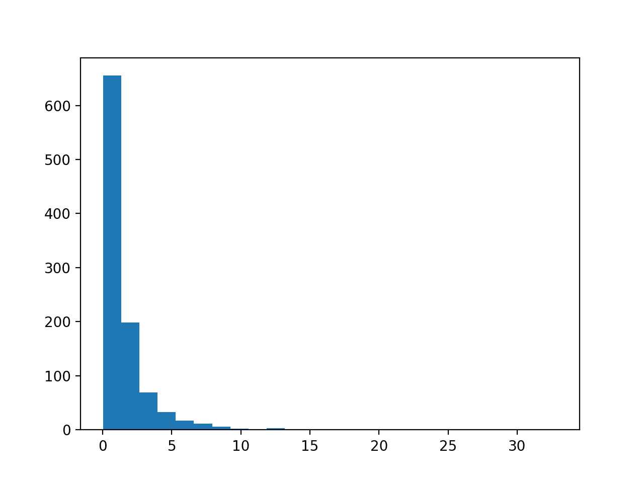
Running the example first creates a sample of 1,000 random Gaussian values and adds a skew to the dataset.
A histogram is created from the skewed dataset and clearly shows the distribution pushed to the far left.
Histogram of Skewed Gaussian Distribution
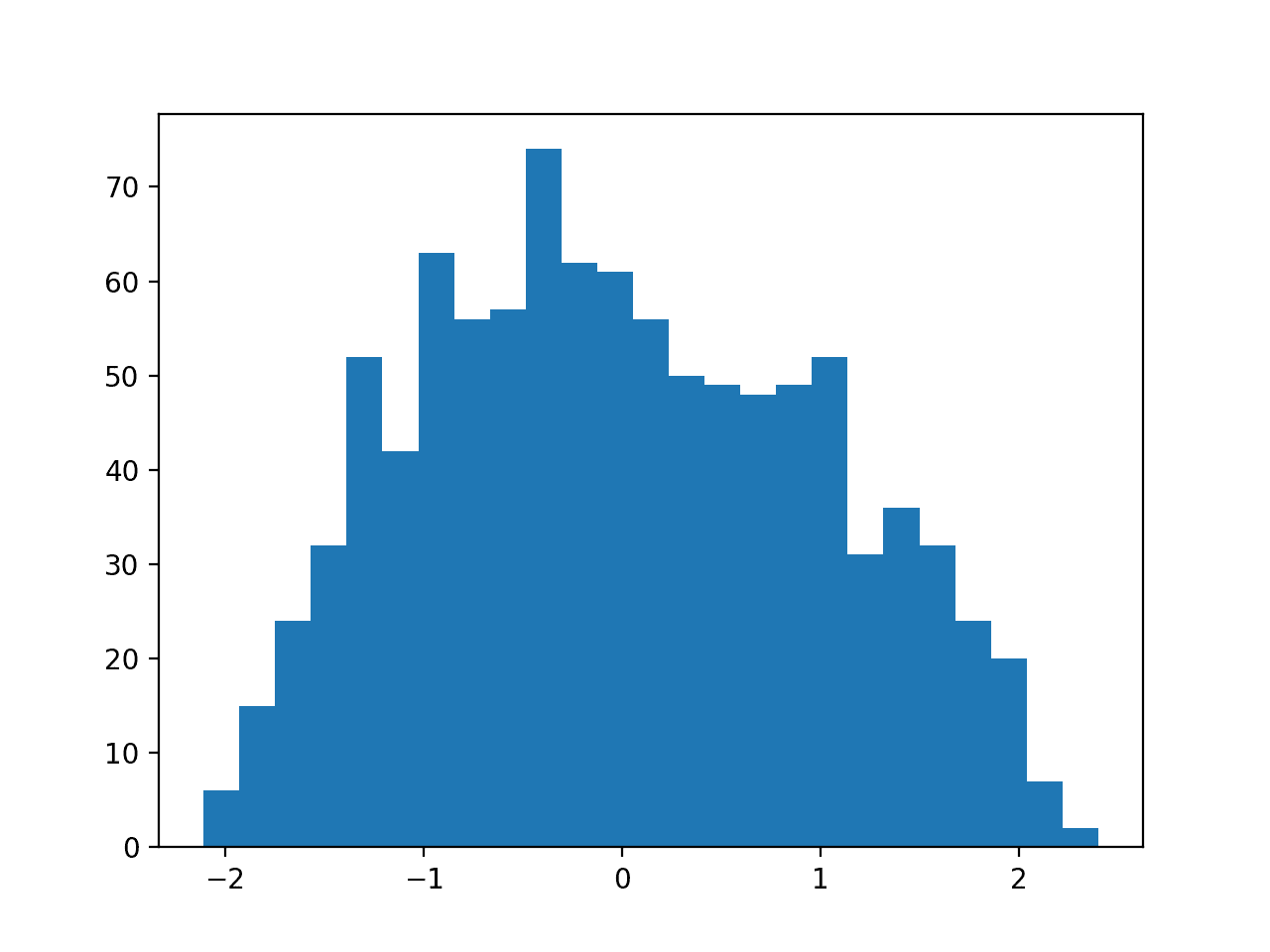
Then a PowerTransformer is used to make the data distribution more-Gaussian and standardize the result, centering the values on the mean value of 0 and a standard deviation of 1.0.
A histogram of the transform data is created showing a more-Gaussian shaped data distribution.
Histogram of Skewed Gaussian Data After Power Transform
In the following sections will take a closer look at how to use these two power transforms on a real dataset.
Next, let’s introduce the dataset.
Sonar Dataset
The sonar dataset is a standard machine learning dataset for binary classification.
It involves 60 real-valued inputs and a 2-class target variable. There are 208 examples in the dataset and the classes are reasonably balanced.
A baseline classification algorithm can achieve a classification accuracy of about 53.4 percent using repeated stratified 10-fold cross-validation. Top performance on this dataset is about 88 percent using repeated stratified 10-fold cross-validation.
The dataset describes radar returns of rocks or simulated mines.
max 0.137100 0.233900 0.305900 ... 0.044000 0.036400 0.043900
[8 rows x 60 columns]
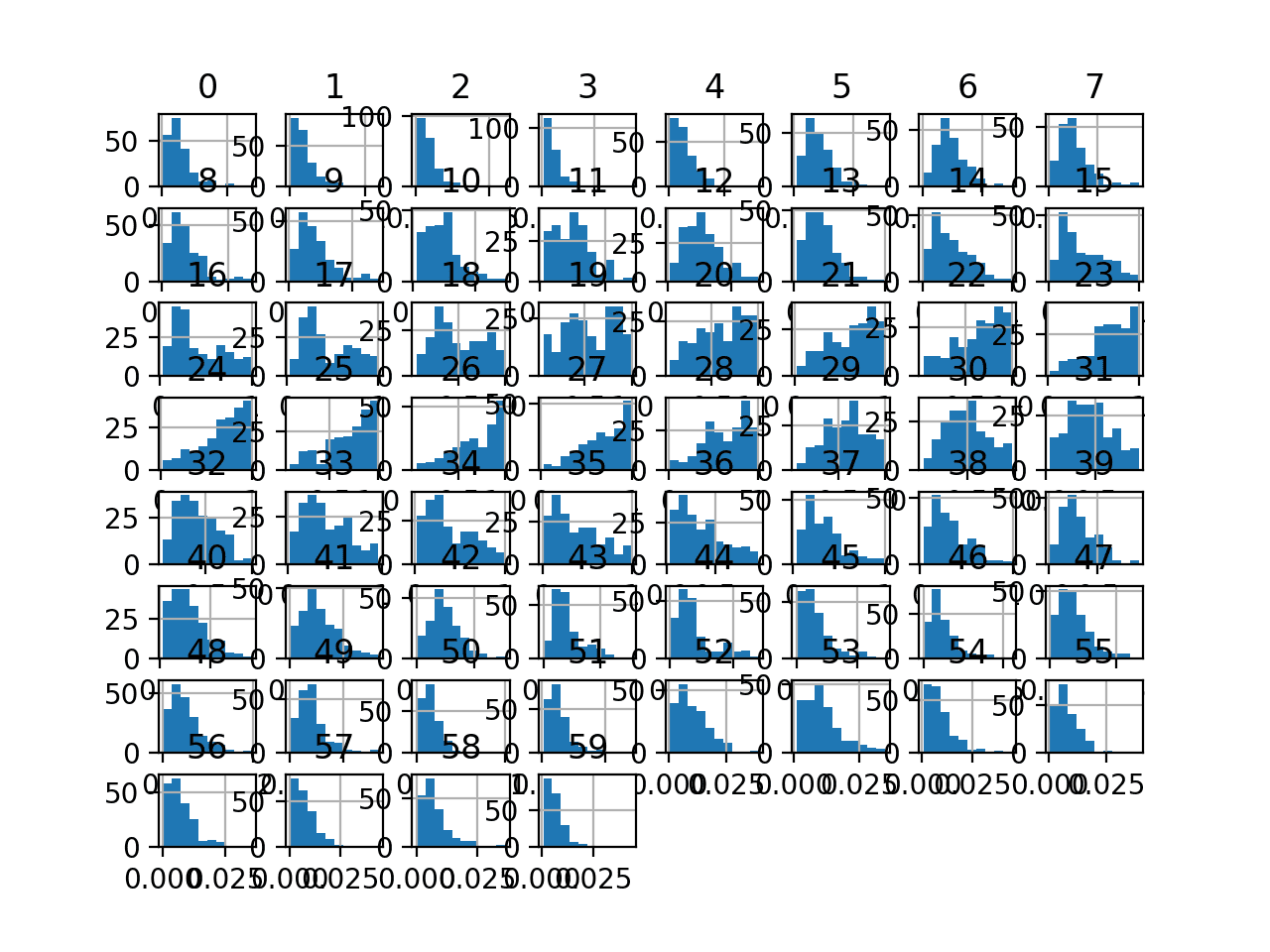
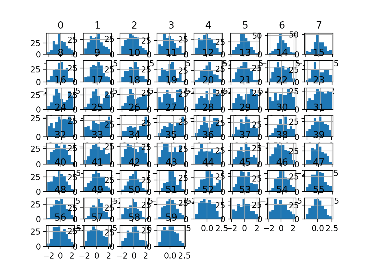
Finally, a histogram is created for each input variable.
If we ignore the clutter of the plots and focus on the histograms themselves, we can see that many variables have a skewed distribution.
The dataset provides a good candidate for using a power transform to make the variables more-Gaussian.
Histogram Plots of Input Variables for the Sonar Binary Classification Dataset
Next, let’s fit and evaluate a machine learning model on the raw dataset.
We will use a k-nearest neighbor algorithm with default hyperparameters and evaluate it using repeated stratified k-fold cross-validation. The complete example is listed below.
1
2
3
4
5
6
7
8
9
10
11
12
13
14
15
16
17
18
19
20
21
22
23
24
25
# evaluate knn on the raw sonar dataset
from numpy import mean
from numpy import std
from pandas import read_csv
from sklearn.model_selection import cross_val_score
from sklearn.model_selection import RepeatedStratifiedKFold
from sklearn.neighbors import KNeighborsClassifier
Running the example evaluates a KNN model on the raw sonar dataset.
Note: Your results may vary given the stochastic nature of the algorithm or evaluation procedure, or differences in numerical precision. Consider running the example a few times and compare the average outcome.
We can see that the model achieved a mean classification accuracy of about 79.7 percent, showing that it has skill (better than 53.4 percent) and is in the ball-park of good performance (88 percent).
1
Accuracy: 0.797 (0.073)
Next, let’s explore a Box-Cox power transform of the dataset.
Box-Cox Transform
The Box-Cox transform is named for the two authors of the method.
It is a power transform that assumes the values of the input variable to which it is applied are strictly positive. That means 0 and negative values are not supported.
It is important to note that the Box-Cox procedure can only be applied to data that is strictly positive.
We can apply the Box-Cox transform using the PowerTransformer class and setting the “method” argument to “box-cox“. Once defined, we can call the fit_transform() function and pass it to our dataset to create a Box-Cox transformed version of our dataset.
1
2
3
...
pt=PowerTransformer(method='box-cox')
data=pt.fit_transform(data)
Our dataset does not have negative values but may have zero values. This may cause a problem.
Let’s try anyway.
The complete example of creating a Box-Cox transform of the sonar dataset and plotting histograms of the result is listed below.
1
2
3
4
5
6
7
8
9
10
11
12
13
14
15
16
17
18
19
# visualize a box-cox transform of the sonar dataset
from pandas import read_csv
from pandas import DataFrame
from pandas.plotting import scatter_matrix
from sklearn.preprocessing import PowerTransformer
Note: Your results may vary given the stochastic nature of the algorithm or evaluation procedure, or differences in numerical precision. Consider running the example a few times and compare the average outcome.
Running the example, we can see that the Box-Cox transform results in a lift in performance from 79.7 percent accuracy without the transform to about 81.1 percent with the transform.
1
Accuracy: 0.811 (0.085)
Next, let’s take a closer look at the Yeo-Johnson transform.
Yeo-Johnson Transform
The Yeo-Johnson transform is also named for the authors.
Unlike the Box-Cox transform, it does not require the values for each input variable to be strictly positive. It supports zero values and negative values. This means we can apply it to our dataset without scaling it first.
We can apply the transform by defining a PowerTransform object and setting the “method” argument to “yeo-johnson” (the default).
1
2
3
4
...
# perform a yeo-johnson transform of the dataset
pt=PowerTransformer(method='yeo-johnson')
data=pt.fit_transform(data)
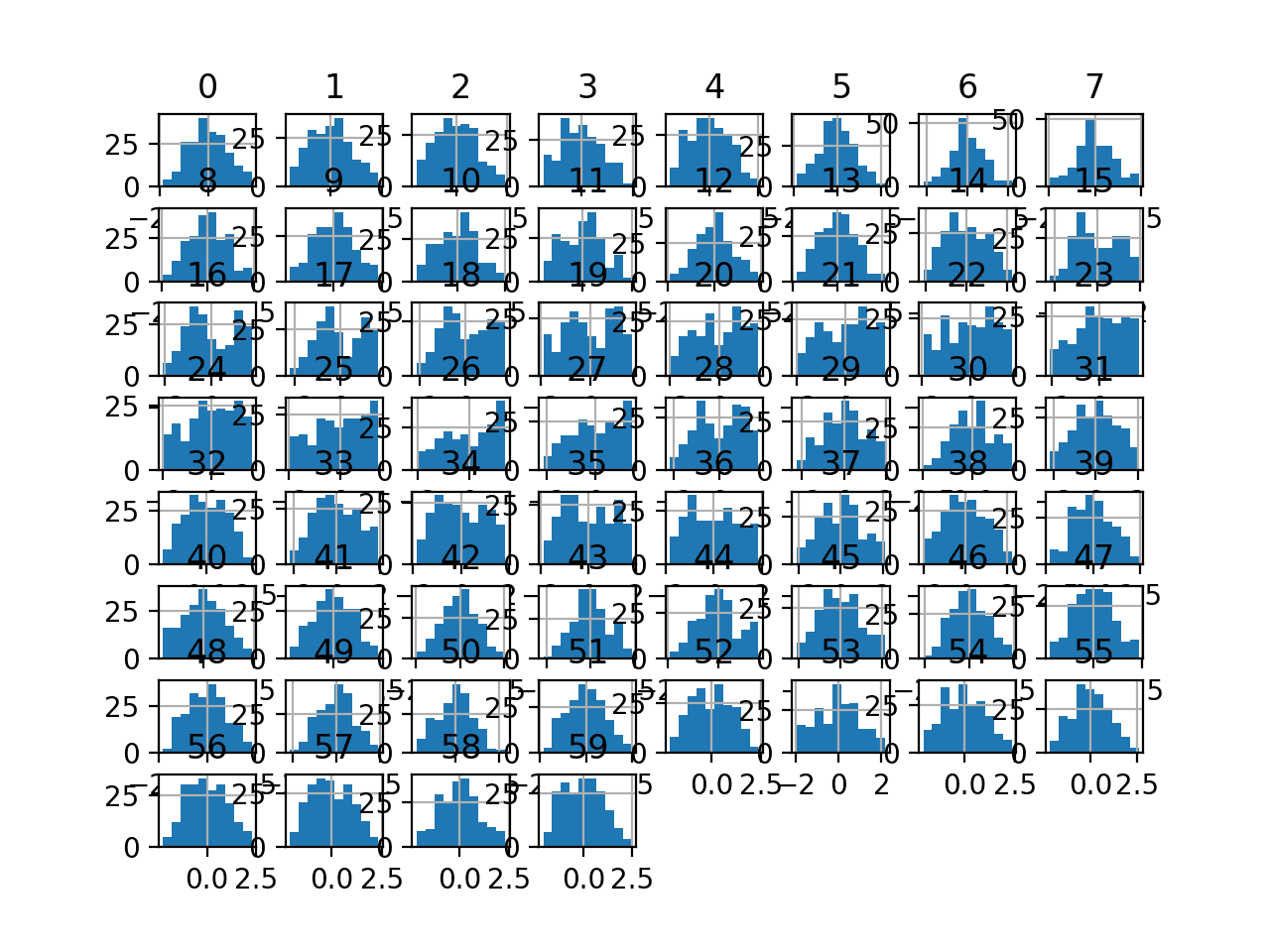
The example below applies the Yeo-Johnson transform and creates histogram plots of each of the transformed variables.
1
2
3
4
5
6
7
8
9
10
11
12
13
14
15
16
17
18
19
# visualize a yeo-johnson transform of the sonar dataset
from pandas import read_csv
from pandas import DataFrame
from pandas.plotting import scatter_matrix
from sklearn.preprocessing import PowerTransformer
Note: Your results may vary given the stochastic nature of the algorithm or evaluation procedure, or differences in numerical precision. Consider running the example a few times and compare the average outcome.
Running the example, we can see that the Yeo-Johnson transform results in a lift in performance from 79.7 percent accuracy without the transform to about 80.8 percent with the transform, less than the Box-Cox transform that achieved about 81.1 percent.
1
Accuracy: 0.808 (0.082)
Sometimes a lift in performance can be achieved by first standardizing the raw dataset prior to performing a Yeo-Johnson transform.
We can explore this by adding a StandardScaler as a first step in the pipeline.
The complete example is listed below.
1
2
3
4
5
6
7
8
9
10
11
12
13
14
15
16
17
18
19
20
21
22
23
24
25
26
27
28
29
30
31
# evaluate knn on the yeo-johnson standardized sonar dataset
from numpy import mean
from numpy import std
from pandas import read_csv
from sklearn.model_selection import cross_val_score
from sklearn.model_selection import RepeatedStratifiedKFold
from sklearn.neighbors import KNeighborsClassifier
from sklearn.preprocessing import LabelEncoder
from sklearn.preprocessing import PowerTransformer
Note: Your results may vary given the stochastic nature of the algorithm or evaluation procedure, or differences in numerical precision. Consider running the example a few times and compare the average outcome.
Running the example, we can see that standardizing the data prior to the Yeo-Johnson transform resulted in a small lift in performance from about 80.8 percent to about 81.6 percent, a small lift over the results for the Box-Cox transform.
1
Accuracy: 0.816 (0.077)
Further Reading
This section provides more resources on the topic if you are looking to go deeper.
In this tutorial, you discovered how to use power transforms in scikit-learn to make variables more Gaussian for modeling.
Specifically, you learned:
Many machine learning algorithms prefer or perform better when numerical variables have a Gaussian probability distribution.
Power transforms are a technique for transforming numerical input or output variables to have a Gaussian or more-Gaussian-like probability distribution.
How to use the PowerTransform in scikit-learn to use the Box-Cox and Yeo-Johnson transforms when preparing data for predictive modeling.
Do you have any questions?
Ask your questions in the comments below and I will do my best to answer.
It provides self-study tutorials with full working code on: Feature Selection, RFE, Data Cleaning, Data Transforms, Scaling, Dimensionality Reduction,
and much more...
Bring Modern Data Preparation Techniques to Your Machine Learning Projects
Hi Jason,
Thanks for this great post.
My question is I see you transform the whole dataset and build model on it.
I am so confused. Does not it have data leakage?
Given MLE is estimating the parameter of P(y | parameter, x), by “assume a Gaussian distribution in the input variables.” you mean the P(x) ~ gaussian?
first at all thank you for touching on this topic, it is quite helpful to see someone hands-on tackling the topic.
I have two questions in mind that came to me in practice when exploring data transformation procedures. Is there any “golden-guide” on what to do first in order to generally have a more robust procedure? With this I mean that, for instance, you applied first scaling and then the data transformation, but similar results can be found doing first the data transformation and afterwards the scaling (I found sometimes better, sometimes worse results, it can vary on different models).
Also, if the data one is using contains negative ore even zero values, boxcox will return “ValueError: The Box-Cox transformation can only be applied to strictly positive data”.
Do you know a way to still use boxcox in the pipeline while dealing with this kind of problems?
Hi, I have applied my Exponential 1d array ‘Yeo-Johnson’ to get more Gaussian data before applying the Kde and splitting my 1d array to 3 cluster. Anyway it worked better but i dont know how to get back my original data values now?)
I am using deep learning for tabular data (regression).
Q1: Shall I transform the target column?
Q2 if yes, then when I deploy a model to give me a new prediction, I will get the target in Transformed way, how I can re-Transform it to original data values?
I got all your ebooks in the last black Friday 🙂 I highly recommend them.
Thank for the amazing work.
fabulous lesson like always. I did enjoy reading it and truly learned a lot. I also read the other two related articles on Quantile Transforms and Discretization Transforms.
I have a silly question about the beginning of the code, is it necessary to transform the Panda’s dataframe to NumPy array (.values)? let’s say if we didn’t, would we get the same results? or it might cause other problems with the transformers?
Thank you again and please keep up the good work,
Regards,
What is the key/unique difference between standardisation and power transform.
I understand that (standardisation is bring to a same scale),(power transform is removing the skewness/variance stabilizing). anything specific and beyond this point? Thanks in advance.
@Sam : It is worth mentioning that both of those transformations keep the monotonicity of the points within a variable. Some ML models like Random Forest are not prone to such transformations, so it is not worth testing/using those data transformations there. However, in case of some Gradient Boosting Trees implementations I can imagine that variable binning approaches may be dependent on power transformation usage.
Regards!
Dear Jason, thanks for this great post, as always!
I was wondering regarding the ‘Box-Cox’ method, In case I only have zero values (and not negative), can I just shift the data by 0.001 or 1 (or whatever…) before the transformation?
instead of using MixMaxScaler transform?
I am using the transformation before applying IterativeImputer (with BayesianRidge estimator), so I need to transform first my data.
Yes, I tried a couple of things. Interestingly the IterativeImputer becomes unstable after a few iterations no matter what transformation I perform. It seems that it gets into some bad feeadback loop of values out of range. The alternative option of not performing any transformation to Normal distribution however generates negative imputed values, which are not physical.
How to power transform back to the original value scale? For example, price is the target variable, and is power transformed to the normal distribution. The modeling is then performed, and the predicted price value needs be transformed back to the real scale using the the underlined transformation function. How should I do it? BTW this is a great post!! thank you!
I have a time series dataset (interval =quarterly; multi-index = (year, quarter), columns=financial aspects (e.g. accounts payables)).
I did NOT provide a lambda value, I let the estimator estimate the lambda parameter.
Some ‘X_columns’ are NOT ok with Yeo-Johnson transformation while those same columns are ok with BoxCox.
After running several times, consistent results are shown below:
Plot of X_column results after Y-J: created a horizontal line (y=0.25), lambda = -3.99
Plot of X_column results after B-C: as expected results, lambda = 0.00232
Q1) Can you provide theoretical reasoning for this difference in outcome?
Q2) Both B-C and Y-J ‘maximizes the log-likelihood function’ to estimate lambda, where is the noise arising from?
Hi Jason. First of all, thanks for your amazing work. I have a doubt in this tutorial: when you introduce the PowerTransformer in the Pipeline, does it transform the target data as well?
I also highly recommend purchasing your courses, they’re worth it!
Sir, i need a favour I have applied quantile transformation to both my features and target parameters for gaussian process regression. But finally, I want to transform back the points during performance calculation. How can I do that? is there any library available for the same?
Could you please explain more about data specifications and domains that can undermine the data validity after transformation for machine learning applications?
Any references on this would also be much appreciated.
Dear Jason,
Thanks for a truly helpful and inspiring blog/website – amazing stuff to read.
With regard to this post and the Box-Cox powertransform I have a question:
Is it possible to only do the Box-Cox transform for selected features in my dataset? Right now I get a valuerror (“Data must not be constant”), due to the fact that my dataset consists of several 0/1-features. Mainly because of the one-hot-encoding transform at the beginning of the pipeline… If it was possible to only do the Box-Cox powertransform for selected features I would be able to have a “clean” pipeline. Or am I missing something simple?


Hello.I understand that there are no assumptions in any linear model about the distribution of the independent variables. Could you clarify that?
Linear models like a linear regression or logistic regression often assume a Gaussian distribution in the input variables.
Hi Jason,
Thanks for this great post.
My question is I see you transform the whole dataset and build model on it.
I am so confused. Does not it have data leakage?
Please advise
We only transform the whole data in this tutorial to show you the effect of the transform.
The modeling example in the tutorial uses a Pipeline to avoid data leakage. If this is a new idea for you, see this:
https://machinelearningmastery.com/data-preparation-without-data-leakage/
Given MLE is estimating the parameter of P(y | parameter, x), by “assume a Gaussian distribution in the input variables.” you mean the P(x) ~ gaussian?
Hi oaixuroab…You are correct! Thank you for the feedback!
Dear Jason,
first at all thank you for touching on this topic, it is quite helpful to see someone hands-on tackling the topic.
I have two questions in mind that came to me in practice when exploring data transformation procedures. Is there any “golden-guide” on what to do first in order to generally have a more robust procedure? With this I mean that, for instance, you applied first scaling and then the data transformation, but similar results can be found doing first the data transformation and afterwards the scaling (I found sometimes better, sometimes worse results, it can vary on different models).
Also, if the data one is using contains negative ore even zero values, boxcox will return “ValueError: The Box-Cox transformation can only be applied to strictly positive data”.
Do you know a way to still use boxcox in the pipeline while dealing with this kind of problems?
Thank you so much in advance.
Thanks!
Yes, scale data to be positive first, I find the range 1 to 2 more stable than 0e+5 to 1.
Hi, I have applied my Exponential 1d array ‘Yeo-Johnson’ to get more Gaussian data before applying the Kde and splitting my 1d array to 3 cluster. Anyway it worked better but i dont know how to get back my original data values now?)
Great!
Hi Jason, Thank you, this is very helpful.
I have 2 questions:
I am using deep learning for tabular data (regression).
Q1: Shall I transform the target column?
Q2 if yes, then when I deploy a model to give me a new prediction, I will get the target in Transformed way, how I can re-Transform it to original data values?
I got all your ebooks in the last black Friday 🙂 I highly recommend them.
Thank for the amazing work.
Try it and see if it results in better performance.
Yes! If you use a pipeline then it will invert the transform for you automatically:
https://machinelearningmastery.com/how-to-transform-target-variables-for-regression-with-scikit-learn/
Thanks!
fabulous lesson like always. I did enjoy reading it and truly learned a lot. I also read the other two related articles on Quantile Transforms and Discretization Transforms.
I have a silly question about the beginning of the code, is it necessary to transform the Panda’s dataframe to NumPy array (.values)? let’s say if we didn’t, would we get the same results? or it might cause other problems with the transformers?
Thank you again and please keep up the good work,
Regards,
Thanks!
No, but I prefer to work with numpy arrays directly.
Perfect, thank you for the response!
You’re welcome.
What is the key/unique difference between standardisation and power transform.
I understand that (standardisation is bring to a same scale),(power transform is removing the skewness/variance stabilizing). anything specific and beyond this point? Thanks in advance.
@Sam : It is worth mentioning that both of those transformations keep the monotonicity of the points within a variable. Some ML models like Random Forest are not prone to such transformations, so it is not worth testing/using those data transformations there. However, in case of some Gradient Boosting Trees implementations I can imagine that variable binning approaches may be dependent on power transformation usage.
Regards!
Not really, you nailed it.
Dear Jason, thanks for this great post, as always!
I was wondering regarding the ‘Box-Cox’ method, In case I only have zero values (and not negative), can I just shift the data by 0.001 or 1 (or whatever…) before the transformation?
instead of using MixMaxScaler transform?
I am using the transformation before applying IterativeImputer (with BayesianRidge estimator), so I need to transform first my data.
Thanks!
Idit
Yes, add a small value or scale to a new positive range.
Try a few methods, see what works well.
Yes, I tried a couple of things. Interestingly the IterativeImputer becomes unstable after a few iterations no matter what transformation I perform. It seems that it gets into some bad feeadback loop of values out of range. The alternative option of not performing any transformation to Normal distribution however generates negative imputed values, which are not physical.
Perhaps use some custom code to clean up imputed values or do imputation manually.
I’ll figure something out… thanks a lot for your advice!
You’re welcome.
How to power transform back to the original value scale? For example, price is the target variable, and is power transformed to the normal distribution. The modeling is then performed, and the predicted price value needs be transformed back to the real scale using the the underlined transformation function. How should I do it? BTW this is a great post!! thank you!
If you transform the target, then you may need to invert the transform on predictions made by the model.
If the transform is on inputs only, no inversion of the transform is needed.
Hi Jason,
I have a time series dataset (interval =quarterly; multi-index = (year, quarter), columns=financial aspects (e.g. accounts payables)).
I did NOT provide a lambda value, I let the estimator estimate the lambda parameter.
Some ‘X_columns’ are NOT ok with Yeo-Johnson transformation while those same columns are ok with BoxCox.
After running several times, consistent results are shown below:
Plot of X_column results after Y-J: created a horizontal line (y=0.25), lambda = -3.99
Plot of X_column results after B-C: as expected results, lambda = 0.00232
Q1) Can you provide theoretical reasoning for this difference in outcome?
Q2) Both B-C and Y-J ‘maximizes the log-likelihood function’ to estimate lambda, where is the noise arising from?
What do you mean a theoretical reasoning? You can perform the calculations manually to see at how the algorithm arrived at the result.
Hi Jason,
Is it better to first scale data and then apply a transformation or vice versa?
You do that in the examples
Thanks a lot
Very useful as usual! 🙂
I forgot to ask one more thing:
in a pipeline with 3 tasks:
A) Smote
B) PowerTransformer
c) MinMaxScaler
In what order should I execute those steps in a pipeline?
Thanks!
Perhaps experiment and see what order results in the best performance for your specific dataset and model.
I would guess minmax, power, then smote.
yes, I tried that and it is better indeed.
Thanks Jason, I really apretiate that 🙂
Well done.
Scale and then transform.
Thanks for putting this up, it totally helps make things clearer
You’re welcome!
Hi Jason. First of all, thanks for your amazing work. I have a doubt in this tutorial: when you introduce the PowerTransformer in the Pipeline, does it transform the target data as well?
I also highly recommend purchasing your courses, they’re worth it!
Thank you
You’re welcome.
No, the pipeline is only applied to the input.
Thanks!!!
Hi, Jason!
It’s such an interesting article!!
Would it be useful to use Power Transforms for Deep Learning as well?
Thanks
Thanks.
Yes!
“Some algorithms like linear regression and logistic regression explicitly assume the real-valued variables have a Gaussian distribution.”
No! Logistic regression doesn’t make the same assumptions of linear regression. The predictors don ‘t need to be normally distributed.
Okay, thanks.
Sir, i need a favour I have applied quantile transformation to both my features and target parameters for gaussian process regression. But finally, I want to transform back the points during performance calculation. How can I do that? is there any library available for the same?
You can call inverse_transform() on the object and pass in the data.
Hi Jason,
Could you please explain to what extent transforming the data to have a Gaussian-like distribution can compromise the validity of the data?
Thanks,
Keyvan
Not really, it may depend on the specifics of the data and domain.
Could you please explain more about data specifications and domains that can undermine the data validity after transformation for machine learning applications?
Any references on this would also be much appreciated.
Thanks,
I would recommend the references listed in the further reading section.
Could you please mention if there is any disadvantages for non-linear transformations? Either power transformers or quantile transformation?
Hi Esmat…the following resource may help in understanding how and when to use power transforms.
https://www.yourdatateacher.com/2021/04/21/when-and-how-to-use-power-transform-in-machine-learning/
thanks alot of iformation
You are very welcome Reyhan!
Do the Yeo-Johnson or Box-Cox risk data leakage if applied to the whole dataset?
Hi Ben…the following may be of interest:
https://machinelearningmastery.com/data-leakage-machine-learning/
Dear Jason,
Thanks for a truly helpful and inspiring blog/website – amazing stuff to read.
With regard to this post and the Box-Cox powertransform I have a question:
Is it possible to only do the Box-Cox transform for selected features in my dataset? Right now I get a valuerror (“Data must not be constant”), due to the fact that my dataset consists of several 0/1-features. Mainly because of the one-hot-encoding transform at the beginning of the pipeline… If it was possible to only do the Box-Cox powertransform for selected features I would be able to have a “clean” pipeline. Or am I missing something simple?
Thanks in advance!
Kind regards,
Mads.
Hi Mads…The following discussion may be of interest to you:
https://stackoverflow.com/questions/62116192/valueerror-data-must-not-be-constant