Datasets may have missing values, and this can cause problems for many machine learning algorithms.
As such, it is good practice to identify and replace missing values for each column in your input data prior to modeling your prediction task. This is called missing data imputation, or imputing for short.
A popular approach for data imputation is to calculate a statistical value for each column (such as a mean) and replace all missing values for that column with the statistic. It is a popular approach because the statistic is easy to calculate using the training dataset and because it often results in good performance.
In this tutorial, you will discover how to use statistical imputation strategies for missing data in machine learning.
After completing this tutorial, you will know:
Missing values must be marked with NaN values and can be replaced with statistical measures to calculate the column of values.
How to load a CSV value with missing values and mark the missing values with NaN values and report the number and percentage of missing values for each column.
How to impute missing values with statistics as a data preparation method when evaluating models and when fitting a final model to make predictions on new data.
Kick-start your project with my new book Data Preparation for Machine Learning, including step-by-step tutorials and the Python source code files for all examples.
Let’s get started.
Updated Jun/2020: Changed the column used for prediction in examples.
Statistical Imputation for Missing Values in Machine Learning Photo by Bernal Saborio, some rights reserved.
Tutorial Overview
This tutorial is divided into three parts; they are:
Statistical Imputation
Horse Colic Dataset
Statistical Imputation With SimpleImputer
SimpleImputer Data Transform
SimpleImputer and Model Evaluation
Comparing Different Imputed Statistics
SimpleImputer Transform When Making a Prediction
Statistical Imputation
A dataset may have missing values.
These are rows of data where one or more values or columns in that row are not present. The values may be missing completely or they may be marked with a special character or value, such as a question mark “?”.
These values can be expressed in many ways. I’ve seen them show up as nothing at all […], an empty string […], the explicit string NULL or undefined or N/A or NaN, and the number 0, among others. No matter how they appear in your dataset, knowing what to expect and checking to make sure the data matches that expectation will reduce problems as you start to use the data.
Values could be missing for many reasons, often specific to the problem domain, and might include reasons such as corrupt measurements or data unavailability.
They may occur for a number of reasons, such as malfunctioning measurement equipment, changes in experimental design during data collection, and collation of several similar but not identical datasets.
Most machine learning algorithms require numeric input values, and a value to be present for each row and column in a dataset. As such, missing values can cause problems for machine learning algorithms.
As such, it is common to identify missing values in a dataset and replace them with a numeric value. This is called data imputing, or missing data imputation.
A simple and popular approach to data imputation involves using statistical methods to estimate a value for a column from those values that are present, then replace all missing values in the column with the calculated statistic.
It is simple because statistics are fast to calculate and it is popular because it often proves very effective.
Common statistics calculated include:
The column mean value.
The column median value.
The column mode value.
A constant value.
Now that we are familiar with statistical methods for missing value imputation, let’s take a look at a dataset with missing values.
Want to Get Started With Data Preparation?
Take my free 7-day email crash course now (with sample code).
Click to sign-up and also get a free PDF Ebook version of the course.
Horse Colic Dataset
The horse colic dataset describes medical characteristics of horses with colic and whether they lived or died.
There are 300 rows and 26 input variables with one output variable. It is a binary classification prediction task that involves predicting 1 if the horse lived and 2 if the horse died.
There are many fields we could select to predict in this dataset. In this case, we will predict whether the problem was surgical or not (column index 23), making it a binary classification problem.
The dataset has numerous missing values for many of the columns where each missing value is marked with a question mark character (“?”).
Below provides an example of rows from the dataset with marked missing values.
4 2.0 1 530255 37.3 104.0 35.0 NaN ... NaN 2.0 2 4300 0 0 2
[5 rows x 28 columns]
Next, we can see the list of all columns in the dataset and the number and percentage of missing values.
We can see that some columns (e.g. column indexes 1 and 2) have no missing values and other columns (e.g. column indexes 15 and 21) have many or even a majority of missing values.
1
2
3
4
5
6
7
8
9
10
11
12
13
14
15
16
17
18
19
20
21
22
23
24
25
26
27
28
> 0, Missing: 1 (0.3%)
> 1, Missing: 0 (0.0%)
> 2, Missing: 0 (0.0%)
> 3, Missing: 60 (20.0%)
> 4, Missing: 24 (8.0%)
> 5, Missing: 58 (19.3%)
> 6, Missing: 56 (18.7%)
> 7, Missing: 69 (23.0%)
> 8, Missing: 47 (15.7%)
> 9, Missing: 32 (10.7%)
> 10, Missing: 55 (18.3%)
> 11, Missing: 44 (14.7%)
> 12, Missing: 56 (18.7%)
> 13, Missing: 104 (34.7%)
> 14, Missing: 106 (35.3%)
> 15, Missing: 247 (82.3%)
> 16, Missing: 102 (34.0%)
> 17, Missing: 118 (39.3%)
> 18, Missing: 29 (9.7%)
> 19, Missing: 33 (11.0%)
> 20, Missing: 165 (55.0%)
> 21, Missing: 198 (66.0%)
> 22, Missing: 1 (0.3%)
> 23, Missing: 0 (0.0%)
> 24, Missing: 0 (0.0%)
> 25, Missing: 0 (0.0%)
> 26, Missing: 0 (0.0%)
> 27, Missing: 0 (0.0%)
Now that we are familiar with the horse colic dataset that has missing values, let’s look at how we can use statistical imputation.
Statistical Imputation With SimpleImputer
The scikit-learn machine learning library provides the SimpleImputer class that supports statistical imputation.
In this section, we will explore how to effectively use the SimpleImputer class.
SimpleImputer Data Transform
The SimpleImputer is a data transform that is first configured based on the type of statistic to calculate for each column, e.g. mean.
1
2
3
...
# define imputer
imputer=SimpleImputer(strategy='mean')
Then the imputer is fit on a dataset to calculate the statistic for each column.
1
2
3
...
# fit on the dataset
imputer.fit(X)
The fit imputer is then applied to a dataset to create a copy of the dataset with all missing values for each column replaced with a statistic value.
1
2
3
...
# transform the dataset
Xtrans=imputer.transform(X)
We can demonstrate its usage on the horse colic dataset and confirm it works by summarizing the total number of missing values in the dataset before and after the transform.
The complete example is listed below.
1
2
3
4
5
6
7
8
9
10
11
12
13
14
15
16
17
18
19
20
21
# statistical imputation transform for the horse colic dataset
Running the example first loads the dataset and reports the total number of missing values in the dataset as 1,605.
The transform is configured, fit, and performed and the resulting new dataset has no missing values, confirming it was performed as we expected.
Each missing value was replaced with the mean value of its column.
1
2
Missing: 1605
Missing: 0
SimpleImputer and Model Evaluation
It is a good practice to evaluate machine learning models on a dataset using k-fold cross-validation.
To correctly apply statistical missing data imputation and avoid data leakage, it is required that the statistics calculated for each column are calculated on the training dataset only, then applied to the train and test sets for each fold in the dataset.
If we are using resampling to select tuning parameter values or to estimate performance, the imputation should be incorporated within the resampling.
This can be achieved by creating a modeling pipeline where the first step is the statistical imputation, then the second step is the model. This can be achieved using the Pipeline class.
For example, the Pipeline below uses a SimpleImputer with a ‘mean‘ strategy, followed by a random forest model.
Running the example correctly applies data imputation to each fold of the cross-validation procedure.
Note: Your results may vary given the stochastic nature of the algorithm or evaluation procedure, or differences in numerical precision. Consider running the example a few times and compare the average outcome.
The pipeline is evaluated using three repeats of 10-fold cross-validation and reports the mean classification accuracy on the dataset as about 86.3 percent, which is a good score.
1
Mean Accuracy: 0.863 (0.054)
Comparing Different Imputed Statistics
How do we know that using a ‘mean‘ statistical strategy is good or best for this dataset?
The answer is that we don’t and that it was chosen arbitrarily.
We can design an experiment to test each statistical strategy and discover what works best for this dataset, comparing the mean, median, mode (most frequent), and constant (0) strategies. The mean accuracy of each approach can then be compared.
The complete example is listed below.
1
2
3
4
5
6
7
8
9
10
11
12
13
14
15
16
17
18
19
20
21
22
23
24
25
26
27
28
29
30
31
32
# compare statistical imputation strategies for the horse colic dataset
from numpy import mean
from numpy import std
from pandas import read_csv
from sklearn.ensemble import RandomForestClassifier
from sklearn.impute import SimpleImputer
from sklearn.model_selection import cross_val_score
from sklearn.model_selection import RepeatedStratifiedKFold
Running the example evaluates each statistical imputation strategy on the horse colic dataset using repeated cross-validation.
Note: Your results may vary given the stochastic nature of the algorithm or evaluation procedure, or differences in numerical precision. Consider running the example a few times and compare the average outcome.
The mean accuracy of each strategy is reported along the way. The results suggest that using a constant value, e.g. 0, results in the best performance of about 88.1 percent, which is an outstanding result.
1
2
3
4
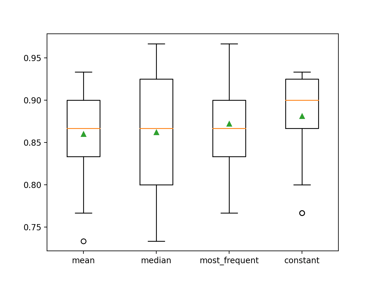
>mean 0.860 (0.054)
>median 0.862 (0.065)
>most_frequent 0.872 (0.052)
>constant 0.881 (0.047)
At the end of the run, a box and whisker plot is created for each set of results, allowing the distribution of results to be compared.
We can clearly see that the distribution of accuracy scores for the constant strategy is better than the other strategies.
Box and Whisker Plot of Statistical Imputation Strategies Applied to the Horse Colic Dataset
SimpleImputer Transform When Making a Prediction
We may wish to create a final modeling pipeline with the constant imputation strategy and random forest algorithm, then make a prediction for new data.
This can be achieved by defining the pipeline and fitting it on all available data, then calling the predict() function passing new data in as an argument.
Importantly, the row of new data must mark any missing values using the NaN value.
In this tutorial, you discovered how to use statistical imputation strategies for missing data in machine learning.
Specifically, you learned:
Missing values must be marked with NaN values and can be replaced with statistical measures to calculate the column of values.
How to load a CSV value with missing values and mark the missing values with NaN values and report the number and percentage of missing values for each column.
How to impute missing values with statistics as a data preparation method when evaluating models and when fitting a final model to make predictions on new data.
Do you have any questions?
Ask your questions in the comments below and I will do my best to answer.
It provides self-study tutorials with full working code on: Feature Selection, RFE, Data Cleaning, Data Transforms, Scaling, Dimensionality Reduction,
and much more...
Bring Modern Data Preparation Techniques to Your Machine Learning Projects
for i in range(dataframe.shape[1]):
# count number of rows with missing values
n_miss = dataframe.isnull().sum()[i] # change this line
perc = n_miss / dataframe.shape[0] * 100
print(‘> %d, Missing: %d (%.1f%%)’ % (i, n_miss, perc))
Hi Jason, great post! Could you please give some intuition why constant imputation gives better results than median/mean imputation? From my point of view it’s unintuitive that so simple technique brings better score than statistical method fitting each individual feature.
We are not good at answering “why” questions in applied machine learning, we don’t have good theories.
I can say something general like it depends on the specifics of the dataset and chosen model. We could dig into the model and figure out why a const results in better performance than a mean for this dataset. It might be a piece of work though.
SimpleImputer class use a single strategy (eg., Mean, median,etc). How do impute missing values in different column with different strategies for a single dataset.in reality, each column may need different strategies to impute missing values.
But I have one query. You are trying filling in 4 statistics for missing values and then validating it based on their respective accuracy. Don’t you think you should focus on finding whether the feature values are normal or non-normal in nature and then impute mean, median respectively. You are focusing on the end result and not doing the right way ? Please correct me if I am wrong.
Hi Jason,
As usual, Another Great post 🙂
Can you give me some details on Model-Based imputation as well, like imputation using KNN or any other machine learning model instead of statistical imputation?
If you can add pro, cons on why model rather statistical or vice-versa that will be more helpful.
Thank you,
Gopi
Hi Sir,
How can I fill missing values in time series data by taking the average of respective month? Do you have any tutorial regarding this in python?
I think the whole idea behind fitting then transforming is indeed to avoid data leakage but this is mainly in the case of K-fold cross-validation. let me explain myself.
In K-fold CV, you are each time fitting or training your model on K-1 folds or subsets then using the one left out to do the validation i.e. measuring the performance of the training model on the validation data.. Then an average of MSEs or MAEs is measured to get the overall model performance.
Now if you have NaN in your dataset and you do imputation the following will happen:
1- You take K-1 folds to train the data
2- You use the left-out fold or subset for validation, but you are considering the left out information in the imputation of the training sets. For example, if mean is used as a strategy for imputation, then you have considered information from the left out dataset to fit your train data. that is by definition data leakage.
I think the same applies to Leave-one-out-cross-validation.
Now the question is ( and that is puzzling me, to be honest ): what about the imputation of NaN in the left-out dataset or the validation dataset? if we use the fit imputation from the training data to fill in NaN for the validation dataset, we are also leaking the data. Since my model will perform better since data from training has leaked to validation.
This gets even worse for the test data if we use the imputer’s fitted to the training data.
This is indeed what the exercise in Kaggle suggests though, so what do I miss here?
You are mentioning in the blog that the sin of preprocessing is for instance doing it before splitting data for validation and testing. Why because we’ll do leakage into training data. But the same happens in the other way round, no?
Suppose I had the NaN values, what would be a better choice for not overperforming my model during testing?
Now the same question with train data fitted imputer and using test data to fill NaN ( say with mean)?
Regardless of the procedure used to evaluate a model (train/test/val, kfold, etc.) a data transform like imputation is fit on the training dataset and applied to all datasets, such as train, test, val, new dataset, etc.
A competition is different as you have the universe of input data available and you can break this rule.
My point is that data leakage happens when unseen data or test data leaks into the training data. That would make the model over-performing.
Then why is this not an issue in the other direction? data leaking from training to test, val etc…
I have not seen any explanation for that? Why is this a rule at all? for me using training data to fit the test data will also make the performance of the model look good on test data.
And why would I need to fit test data with train data at all? isn’t better to fit it with its own data?
The training dataset represents “what is known” prior to making a prediction. A system can and should make complete use of this data in any and all ways prior to making a prediction.
Yes absolutely but in our case, the test data is “known” 🙂
I think the whole idea is that in real life when we’re using new data to predict then we should use the training data for fitting NaN or preprocessing for two main reasons:
1- If we have 1 single observation then preprocessing with it is impracticable
2- usually, new data is “smaller” than train data so the strategy is best estimated with train data be it mean, median etc…plus we’ll be unfair with the model if we fit the test data with itself as this will fill in biased values for the NaN.
What cofounded me is that in competitions, we have a large chunk of the data already available at hands which should in practice well estimate the mean, median etc…
How did you find that the constant imputation strategy according to the whisker plot? what is the empty circle in the plot is it an outlier or something else?
why you always use random-forest classifier for evaluating imputation? is there any point for this algorithm rather than others?
Any data preparation must be fit on the training dataset only, then applied to the train and test sets to avoid data leakage. Or you can use a pipeline that will do this automatically.
however, when i try to implement this on my datasets, when i get to the validation it returns an error ‘ValueError: Input contains NaN, infinity or a value too large for dtype(‘float64′).’ i think X/Y still have NAN values
As a statistician with some expertise in imputation, I would caution your readers against using simple mean inputation. Simply replacing missing values with the mean, is fraught with issues, including, but not limited to:
1. Bias – f the data is not missing completely at random (MCAR), mean imputation can introduce bias into the dataset, as it does not account for the underlying distribution of the data.
2. Artificially Reduces Variability – Imputing with the mean tends to reduce the variability of the dataset, as it replaces missing values with a constant. This can lead to underestimating standard deviation and other measures of spread.
3. Assumes Homogeneous Missingness – Mean imputation does not consider the relationships between different variables, and assumes a homogeneous relationship between the values missingness and other variables in the dataset. Often times, however, missingness is correlated with other variables.
4. Doesn’t Reflect Uncertainty – Mean imputation does not account for the uncertainty associated with the missing values. It treats all imputed values as known, which can lead to smaller standard errors and can result in incorrect conclusions from statistical tests performed on the imputed data.
5. Potential for Overfitting – If mean imputation is used in the context of predictive modeling, it can lead to overfitting, as the model may learn from the artificial structure created by the imputed values.
6. Impact on Correlations – Using the mean can distort correlations between variables, as it can artificially inflate the relationships by homogenizing the values.
Rather than using a constant imputation, I would encourage readers to use a statistically sound approach for imputation such as multiple imputation, or other methods like hot/cold deck imputation. fractional hot deck imputation, or nearest neighbor ratio imputation. Once could even get more complex and use imputation methods like the one described in Semiparametric imputation using latent sparse conditional Gaussian mixtures for multivariate mixed outcomes by S Sugasawa, JK Kim, and K Morikawa (2021)


Hi,
Trying to get the the missing values that are marked with a “?” be replaced with NaN values but I get an error message;
……….
…………….
KeyError: “None of [Int64Index([0], dtype=’int64′)] are in the [columns]”
Please help.
Thanks
Sorry to hear that, are you able to confirm that your libraries are up to date, that you copied the code exactly and that you used the same dataset?
More suggestions here:
https://machinelearningmastery.com/faq/single-faq/why-does-the-code-in-the-tutorial-not-work-for-me
for i in range(dataframe.shape[1]):
# count number of rows with missing values
n_miss = dataframe.isnull().sum()[i] # change this line
perc = n_miss / dataframe.shape[0] * 100
print(‘> %d, Missing: %d (%.1f%%)’ % (i, n_miss, perc))
change this line like that,
n_miss = dataframe.isnull().sum()[i] # change this line
Hi Jason, great post! Could you please give some intuition why constant imputation gives better results than median/mean imputation? From my point of view it’s unintuitive that so simple technique brings better score than statistical method fitting each individual feature.
We are not good at answering “why” questions in applied machine learning, we don’t have good theories.
I can say something general like it depends on the specifics of the dataset and chosen model. We could dig into the model and figure out why a const results in better performance than a mean for this dataset. It might be a piece of work though.
Great post!
Thanks!
Good work!.
So insightful,
Thanks!
SimpleImputer class use a single strategy (eg., Mean, median,etc). How do impute missing values in different column with different strategies for a single dataset.in reality, each column may need different strategies to impute missing values.
Great question!
You can split off each column/feature and prepare any way you wish, then combine the prepared columns back into a dataset to fit/evaluate a model.
A helpful approach might be to use the ColumnTransformer:
https://machinelearningmastery.com/columntransformer-for-numerical-and-categorical-data/
Hi Jason!
Nice Article!
But I have one query. You are trying filling in 4 statistics for missing values and then validating it based on their respective accuracy. Don’t you think you should focus on finding whether the feature values are normal or non-normal in nature and then impute mean, median respectively. You are focusing on the end result and not doing the right way ? Please correct me if I am wrong.
Thanks!
Perhaps. Grid searching different imputation strategies may be faster than understanding the distribution of each variable.
Hi Jason,
As usual, Another Great post 🙂
Can you give me some details on Model-Based imputation as well, like imputation using KNN or any other machine learning model instead of statistical imputation?
If you can add pro, cons on why model rather statistical or vice-versa that will be more helpful.
Thank you,
Gopi
Yes, see this:
https://machinelearningmastery.com/knn-imputation-for-missing-values-in-machine-learning/
Hi Sir,
How can I fill missing values in time series data by taking the average of respective month? Do you have any tutorial regarding this in python?
This might help:
https://machinelearningmastery.com/handle-missing-timesteps-sequence-prediction-problems-python/
I think the whole idea behind fitting then transforming is indeed to avoid data leakage but this is mainly in the case of K-fold cross-validation. let me explain myself.
In K-fold CV, you are each time fitting or training your model on K-1 folds or subsets then using the one left out to do the validation i.e. measuring the performance of the training model on the validation data.. Then an average of MSEs or MAEs is measured to get the overall model performance.
Now if you have NaN in your dataset and you do imputation the following will happen:
1- You take K-1 folds to train the data
2- You use the left-out fold or subset for validation, but you are considering the left out information in the imputation of the training sets. For example, if mean is used as a strategy for imputation, then you have considered information from the left out dataset to fit your train data. that is by definition data leakage.
I think the same applies to Leave-one-out-cross-validation.
Now the question is ( and that is puzzling me, to be honest ): what about the imputation of NaN in the left-out dataset or the validation dataset? if we use the fit imputation from the training data to fill in NaN for the validation dataset, we are also leaking the data. Since my model will perform better since data from training has leaked to validation.
This gets even worse for the test data if we use the imputer’s fitted to the training data.
This is indeed what the exercise in Kaggle suggests though, so what do I miss here?
You are mentioning in the blog that the sin of preprocessing is for instance doing it before splitting data for validation and testing. Why because we’ll do leakage into training data. But the same happens in the other way round, no?
Suppose I had the NaN values, what would be a better choice for not overperforming my model during testing?
Now the same question with train data fitted imputer and using test data to fill NaN ( say with mean)?
Sorry, I don’t follow this question, can you please rephrase or elaborate?
Regardless of the procedure used to evaluate a model (train/test/val, kfold, etc.) a data transform like imputation is fit on the training dataset and applied to all datasets, such as train, test, val, new dataset, etc.
A competition is different as you have the universe of input data available and you can break this rule.
My point is that data leakage happens when unseen data or test data leaks into the training data. That would make the model over-performing.
Then why is this not an issue in the other direction? data leaking from training to test, val etc…
I have not seen any explanation for that? Why is this a rule at all? for me using training data to fit the test data will also make the performance of the model look good on test data.
And why would I need to fit test data with train data at all? isn’t better to fit it with its own data?
The training dataset represents “what is known” prior to making a prediction. A system can and should make complete use of this data in any and all ways prior to making a prediction.
This is the premise of inductive learning / reasoning:
https://en.wikipedia.org/wiki/Inductive_reasoning
Yes absolutely but in our case, the test data is “known” 🙂
I think the whole idea is that in real life when we’re using new data to predict then we should use the training data for fitting NaN or preprocessing for two main reasons:
1- If we have 1 single observation then preprocessing with it is impracticable
2- usually, new data is “smaller” than train data so the strategy is best estimated with train data be it mean, median etc…plus we’ll be unfair with the model if we fit the test data with itself as this will fill in biased values for the NaN.
What cofounded me is that in competitions, we have a large chunk of the data already available at hands which should in practice well estimate the mean, median etc…
Thanks anyway for your feedback 🙂
A competition is not a “real life” situation, and the normal good practices of model evaluation may not be relevant.
For example, you can do crazy stuff like train to the test set:
https://machinelearningmastery.com/train-to-the-test-set-in-machine-learning/
And hill climb the test set:
https://machinelearningmastery.com/hill-climb-the-test-set-for-machine-learning/
Wow that’s insane indeed 🙂
thanks for the information!
You’re welcome.
Dear Jason
can you please explain more about your box plot?
How did you find that the constant imputation strategy according to the whisker plot? what is the empty circle in the plot is it an outlier or something else?
why you always use random-forest classifier for evaluating imputation? is there any point for this algorithm rather than others?
thanks
By default, the constant strategy fills with the value 0, you can learn more here:
https://scikit-learn.org/stable/modules/generated/sklearn.impute.SimpleImputer.html
A dot on a boxplot indicates an outlier:
https://en.wikipedia.org/wiki/Box_plot
I used random forest in this tutorial because it works well on a ton of different problems. Use the algorithm that works best for your dataset.
Hi,
when is the best time to handle missing data if you have categorical features in the dataset,?
Before converting categorical features to numerical or after?
It does not matter really, as long as you don’t allow data leakage. Perhaps after ordinal encoding.
hi, thanks for the reply
Encoding must perform also to training data to avoid data leakage? or data leakage is relevant to the other data preparation techniques?
Any data preparation must be fit on the training dataset only, then applied to the train and test sets to avoid data leakage. Or you can use a pipeline that will do this automatically.
Hi,
Thanks for great post.
Imputation of missing values should be done after removing outlier or before outlier treatment?
Perhaps after. Experiment and discover what works well or best for your specific dataset and models.
HI
Thanks for the information.
however, when i try to implement this on my datasets, when i get to the validation it returns an error ‘ValueError: Input contains NaN, infinity or a value too large for dtype(‘float64′).’ i think X/Y still have NAN values
Maybe your Y has some zero so X/Y gets NaN? Try to do some preprocessing to replace those values before you use it.
Great Post, Thank you Jason
You are very welcome! We greatly appreciate your support!
Jason is erroneus data can categorize as missing values, and how we can handle with it , Thank you in advance
Why do we need to make the missing values for the new data as NaN when the model was trained on the missing values being t a constant 0?
Hi itsme…There are many approaches to handling missing data. The following resource may be of interest:
https://machinelearningmastery.com/handle-missing-data-python/
As a statistician with some expertise in imputation, I would caution your readers against using simple mean inputation. Simply replacing missing values with the mean, is fraught with issues, including, but not limited to:
1. Bias – f the data is not missing completely at random (MCAR), mean imputation can introduce bias into the dataset, as it does not account for the underlying distribution of the data.
2. Artificially Reduces Variability – Imputing with the mean tends to reduce the variability of the dataset, as it replaces missing values with a constant. This can lead to underestimating standard deviation and other measures of spread.
3. Assumes Homogeneous Missingness – Mean imputation does not consider the relationships between different variables, and assumes a homogeneous relationship between the values missingness and other variables in the dataset. Often times, however, missingness is correlated with other variables.
4. Doesn’t Reflect Uncertainty – Mean imputation does not account for the uncertainty associated with the missing values. It treats all imputed values as known, which can lead to smaller standard errors and can result in incorrect conclusions from statistical tests performed on the imputed data.
5. Potential for Overfitting – If mean imputation is used in the context of predictive modeling, it can lead to overfitting, as the model may learn from the artificial structure created by the imputed values.
6. Impact on Correlations – Using the mean can distort correlations between variables, as it can artificially inflate the relationships by homogenizing the values.
Rather than using a constant imputation, I would encourage readers to use a statistically sound approach for imputation such as multiple imputation, or other methods like hot/cold deck imputation. fractional hot deck imputation, or nearest neighbor ratio imputation. Once could even get more complex and use imputation methods like the one described in Semiparametric imputation using latent sparse conditional Gaussian mixtures for multivariate mixed outcomes by S Sugasawa, JK Kim, and K Morikawa (2021)
Thank you Mark for your contribution to our discussion!