Reducing the number of input variables for a predictive model is referred to as dimensionality reduction.
Fewer input variables can result in a simpler predictive model that may have better performance when making predictions on new data.
Linear Discriminant Analysis, or LDA for short, is a predictive modeling algorithm for multi-class classification. It can also be used as a dimensionality reduction technique, providing a projection of a training dataset that best separates the examples by their assigned class.
The ability to use Linear Discriminant Analysis for dimensionality reduction often surprises most practitioners.
In this tutorial, you will discover how to use LDA for dimensionality reduction when developing predictive models.
After completing this tutorial, you will know:
- Dimensionality reduction involves reducing the number of input variables or columns in modeling data.
- LDA is a technique for multi-class classification that can be used to automatically perform dimensionality reduction.
- How to evaluate predictive models that use an LDA projection as input and make predictions with new raw data.
Kick-start your project with my new book Data Preparation for Machine Learning, including step-by-step tutorials and the Python source code files for all examples.
Let’s get started.
- Update May/2020: Improved code commenting

Linear Discriminant Analysis for Dimensionality Reduction in Python
Photo by Kimberly Vardeman, some rights reserved.
Tutorial Overview
This tutorial is divided into four parts; they are:
- Dimensionality Reduction
- Linear Discriminant Analysis
- LDA Scikit-Learn API
- Worked Example of LDA for Dimensionality
Dimensionality Reduction
Dimensionality reduction refers to reducing the number of input variables for a dataset.
If your data is represented using rows and columns, such as in a spreadsheet, then the input variables are the columns that are fed as input to a model to predict the target variable. Input variables are also called features.
We can consider the columns of data representing dimensions on an n-dimensional feature space and the rows of data as points in that space. This is a useful geometric interpretation of a dataset.
In a dataset with k numeric attributes, you can visualize the data as a cloud of points in k-dimensional space …
— Page 305, Data Mining: Practical Machine Learning Tools and Techniques, 4th edition, 2016.
Having a large number of dimensions in the feature space can mean that the volume of that space is very large, and in turn, the points that we have in that space (rows of data) often represent a small and non-representative sample.
This can dramatically impact the performance of machine learning algorithms fit on data with many input features, generally referred to as the “curse of dimensionality.”
Therefore, it is often desirable to reduce the number of input features. This reduces the number of dimensions of the feature space, hence the name “dimensionality reduction.”
A popular approach to dimensionality reduction is to use techniques from the field of linear algebra. This is often called “feature projection” and the algorithms used are referred to as “projection methods.”
Projection methods seek to reduce the number of dimensions in the feature space whilst also preserving the most important structure or relationships between the variables observed in the data.
When dealing with high dimensional data, it is often useful to reduce the dimensionality by projecting the data to a lower dimensional subspace which captures the “essence” of the data. This is called dimensionality reduction.
— Page 11, Machine Learning: A Probabilistic Perspective, 2012.
The resulting dataset, the projection, can then be used as input to train a machine learning model.
In essence, the original features no longer exist and new features are constructed from the available data that are not directly comparable to the original data, e.g. don’t have column names.
Any new data that is fed to the model in the future when making predictions, such as test dataset and new datasets, must also be projected using the same technique.
Want to Get Started With Data Preparation?
Take my free 7-day email crash course now (with sample code).
Click to sign-up and also get a free PDF Ebook version of the course.
Linear Discriminant Analysis
Linear Discriminant Analysis, or LDA, is a linear machine learning algorithm used for multi-class classification.
It should not be confused with “Latent Dirichlet Allocation” (LDA), which is also a dimensionality reduction technique for text documents.
Linear Discriminant Analysis seeks to best separate (or discriminate) the samples in the training dataset by their class value. Specifically, the model seeks to find a linear combination of input variables that achieves the maximum separation for samples between classes (class centroids or means) and the minimum separation of samples within each class.
… find the linear combination of the predictors such that the between-group variance was maximized relative to the within-group variance. […] find the combination of the predictors that gave maximum separation between the centers of the data while at the same time minimizing the variation within each group of data.
— Page 289, Applied Predictive Modeling, 2013.
There are many ways to frame and solve LDA; for example, it is common to describe the LDA algorithm in terms of Bayes Theorem and conditional probabilities.
In practice, LDA for multi-class classification is typically implemented using the tools from linear algebra, and like PCA, uses matrix factorization at the core of the technique. As such, it is good practice to perhaps standardize the data prior to fitting an LDA model.
For more information on how LDA is calculated in detail, see the tutorial:
Now that we are familiar with dimensionality reduction and LDA, let’s look at how we can use this approach with the scikit-learn library.
LDA Scikit-Learn API
We can use LDA to calculate a projection of a dataset and select a number of dimensions or components of the projection to use as input to a model.
The scikit-learn library provides the LinearDiscriminantAnalysis class that can be fit on a dataset and used to transform a training dataset and any additional dataset in the future.
For example:
|
1 2 3 4 5 6 7 8 9 |
... # prepare dataset data = ... # define transform lda = LinearDiscriminantAnalysis() # prepare transform on dataset lda.fit(data) # apply transform to dataset transformed = lda.transform(data) |
The outputs of the LDA can be used as input to train a model.
Perhaps the best approach is to use a Pipeline where the first step is the LDA transform and the next step is the learning algorithm that takes the transformed data as input.
|
1 2 3 4 |
... # define the pipeline steps = [('lda', LinearDiscriminantAnalysis()), ('m', GaussianNB())] model = Pipeline(steps=steps) |
It can also be a good idea to standardize data prior to performing the LDA transform if the input variables have differing units or scales; for example:
|
1 2 3 4 |
... # define the pipeline steps = [('s', StandardScaler()), ('lda', LinearDiscriminantAnalysis()), ('m', GaussianNB())] model = Pipeline(steps=steps) |
Now that we are familiar with the LDA API, let’s look at a worked example.
Worked Example of LDA for Dimensionality
First, we can use the make_classification() function to create a synthetic 10-class classification problem with 1,000 examples and 20 input features, 15 inputs of which are meaningful.
The complete example is listed below.
|
1 2 3 4 5 6 |
# test classification dataset from sklearn.datasets import make_classification # define dataset X, y = make_classification(n_samples=1000, n_features=20, n_informative=15, n_redundant=5, random_state=7, n_classes=10) # summarize the dataset print(X.shape, y.shape) |
Running the example creates the dataset and summarizes the shape of the input and output components.
|
1 |
(1000, 20) (1000,) |
Next, we can use dimensionality reduction on this dataset while fitting a naive Bayes model.
We will use a Pipeline where the first step performs the LDA transform and selects the five most important dimensions or components, then fits a Naive Bayes model on these features. We don’t need to standardize the variables on this dataset, as all variables have the same scale by design.
The pipeline will be evaluated using repeated stratified cross-validation with three repeats and 10 folds per repeat. Performance is presented as the mean classification accuracy.
The complete example is listed below.
|
1 2 3 4 5 6 7 8 9 10 11 12 13 14 15 16 17 18 19 |
# evaluate lda with naive bayes algorithm for classification from numpy import mean from numpy import std from sklearn.datasets import make_classification from sklearn.model_selection import cross_val_score from sklearn.model_selection import RepeatedStratifiedKFold from sklearn.pipeline import Pipeline from sklearn.discriminant_analysis import LinearDiscriminantAnalysis from sklearn.naive_bayes import GaussianNB # define dataset X, y = make_classification(n_samples=1000, n_features=20, n_informative=15, n_redundant=5, random_state=7, n_classes=10) # define the pipeline steps = [('lda', LinearDiscriminantAnalysis(n_components=5)), ('m', GaussianNB())] model = Pipeline(steps=steps) # evaluate model cv = RepeatedStratifiedKFold(n_splits=10, n_repeats=3, random_state=1) n_scores = cross_val_score(model, X, y, scoring='accuracy', cv=cv, n_jobs=-1, error_score='raise') # report performance print('Accuracy: %.3f (%.3f)' % (mean(n_scores), std(n_scores))) |
Running the example evaluates the model and reports the classification accuracy.
Note: Your results may vary given the stochastic nature of the algorithm or evaluation procedure, or differences in numerical precision. Consider running the example a few times and compare the average outcome.
In this case, we can see that the LDA transform with naive bayes achieved a performance of about 31.4 percent.
|
1 |
Accuracy: 0.314 (0.049) |
How do we know that reducing 20 dimensions of input down to five is good or the best we can do?
We don’t; five was an arbitrary choice.
A better approach is to evaluate the same transform and model with different numbers of input features and choose the number of features (amount of dimensionality reduction) that results in the best average performance.
LDA is limited in the number of components used in the dimensionality reduction to between the number of classes minus one, in this case, (10 – 1) or 9
The example below performs this experiment and summarizes the mean classification accuracy for each configuration.
|
1 2 3 4 5 6 7 8 9 10 11 12 13 14 15 16 17 18 19 20 21 22 23 24 25 26 27 28 29 30 31 32 33 34 35 36 37 38 39 40 41 42 43 44 |
# compare lda number of components with naive bayes algorithm for classification from numpy import mean from numpy import std from sklearn.datasets import make_classification from sklearn.model_selection import cross_val_score from sklearn.model_selection import RepeatedStratifiedKFold from sklearn.pipeline import Pipeline from sklearn.discriminant_analysis import LinearDiscriminantAnalysis from sklearn.naive_bayes import GaussianNB from matplotlib import pyplot # get the dataset def get_dataset(): X, y = make_classification(n_samples=1000, n_features=20, n_informative=15, n_redundant=5, random_state=7, n_classes=10) return X, y # get a list of models to evaluate def get_models(): models = dict() for i in range(1,10): steps = [('lda', LinearDiscriminantAnalysis(n_components=i)), ('m', GaussianNB())] models[str(i)] = Pipeline(steps=steps) return models # evaluate a give model using cross-validation def evaluate_model(model, X, y): cv = RepeatedStratifiedKFold(n_splits=10, n_repeats=3, random_state=1) scores = cross_val_score(model, X, y, scoring='accuracy', cv=cv, n_jobs=-1, error_score='raise') return scores # define dataset X, y = get_dataset() # get the models to evaluate models = get_models() # evaluate the models and store results results, names = list(), list() for name, model in models.items(): scores = evaluate_model(model, X, y) results.append(scores) names.append(name) print('>%s %.3f (%.3f)' % (name, mean(scores), std(scores))) # plot model performance for comparison pyplot.boxplot(results, labels=names, showmeans=True) pyplot.show() |
Running the example first reports the classification accuracy for each number of components or features selected.
Note: Your results may vary given the stochastic nature of the algorithm or evaluation procedure, or differences in numerical precision. Consider running the example a few times and compare the average outcome.
We can see a general trend of increased performance as the number of dimensions is increased. On this dataset, the results suggest a trade-off in the number of dimensions vs. the classification accuracy of the model.
The results suggest using the default of nine components achieves the best performance on this dataset, although with a gentle trade-off as fewer dimensions are used.
|
1 2 3 4 5 6 7 8 9 |
>1 0.182 (0.032) >2 0.235 (0.036) >3 0.267 (0.038) >4 0.303 (0.037) >5 0.314 (0.049) >6 0.314 (0.040) >7 0.329 (0.042) >8 0.343 (0.045) >9 0.358 (0.056) |
A box and whisker plot is created for the distribution of accuracy scores for each configured number of dimensions.
We can see the trend of increasing classification accuracy with the number of components, with a limit at nine.
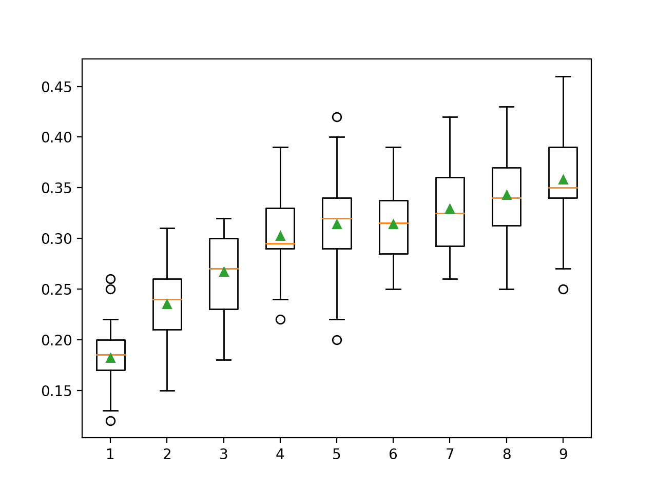
Box Plot of LDA Number of Components vs. Classification Accuracy
We may choose to use an LDA transform and Naive Bayes model combination as our final model.
This involves fitting the Pipeline on all available data and using the pipeline to make predictions on new data. Importantly, the same transform must be performed on this new data, which is handled automatically via the Pipeline.
The code below provides an example of fitting and using a final model with LDA transforms on new data.
|
1 2 3 4 5 6 7 8 9 10 11 12 13 14 15 16 |
# make predictions using lda with naive bayes from sklearn.datasets import make_classification from sklearn.pipeline import Pipeline from sklearn.discriminant_analysis import LinearDiscriminantAnalysis from sklearn.naive_bayes import GaussianNB # define dataset X, y = make_classification(n_samples=1000, n_features=20, n_informative=15, n_redundant=5, random_state=7, n_classes=10) # define the model steps = [('lda', LinearDiscriminantAnalysis(n_components=9)), ('m', GaussianNB())] model = Pipeline(steps=steps) # fit the model on the whole dataset model.fit(X, y) # make a single prediction row = [[2.3548775,-1.69674567,1.6193882,-1.19668862,-2.85422348,-2.00998376,16.56128782,2.57257575,9.93779782,0.43415008,6.08274911,2.12689336,1.70100279,3.32160983,13.02048541,-3.05034488,2.06346747,-3.33390362,2.45147541,-1.23455205]] yhat = model.predict(row) print('Predicted Class: %d' % yhat[0]) |
Running the example fits the Pipeline on all available data and makes a prediction on new data.
Here, the transform uses the nine most important components from the LDA transform as we found from testing above.
A new row of data with 20 columns is provided and is automatically transformed to 15 components and fed to the naive bayes model in order to predict the class label.
|
1 |
Predicted Class: 6 |
Further Reading
This section provides more resources on the topic if you are looking to go deeper.
Tutorials
Books
- Machine Learning: A Probabilistic Perspective, 2012.
- Data Mining: Practical Machine Learning Tools and Techniques, 4th edition, 2016.
- Pattern Recognition and Machine Learning, 2006.
- Applied Predictive Modeling, 2013.
APIs
- Decomposing signals in components (matrix factorization problems), scikit-learn.
- sklearn.discriminant_analysis.LinearDiscriminantAnalysis API.
- sklearn.pipeline.Pipeline API.
Articles
- Dimensionality reduction, Wikipedia.
- Curse of dimensionality, Wikipedia.
- Linear discriminant analysis, Wikipedia.
Summary
In this tutorial, you discovered how to use LDA for dimensionality reduction when developing predictive models.
Specifically, you learned:
- Dimensionality reduction involves reducing the number of input variables or columns in modeling data.
- LDA is a technique for multi-class classification that can be used to automatically perform dimensionality reduction.
- How to evaluate predictive models that use an LDA projection as input and make predictions with new raw data.
Do you have any questions?
Ask your questions in the comments below and I will do my best to answer.
Get a Handle on Modern Data Preparation!

Prepare Your Machine Learning Data in Minutes
...with just a few lines of python code
Discover how in my new Ebook:
Data Preparation for Machine Learning
It provides self-study tutorials with full working code on:
Feature Selection, RFE, Data Cleaning, Data Transforms, Scaling, Dimensionality Reduction,
and much more...


Can I know that in the context of dimensionality reduction using LDA/FDA. (Not for prediction)
The output is “c-1” where “c” is the number of classes and the dimensionality of the data is n with “n>c”.
Let say my original dataset has 2 classes, the output will be 1 dimensionality ( 2 – 1 =1 ), likewise, if my original dataset has 5 classes, the output will be 4 dimensionality.
The output tis whatever you choose to configure the LDA to produce – as we see in the above tutorial.
Dear Dr Jason,
In the following code from the above:
My question is about the
If n_components= 5, does the LDA select the first 5 features generated by make_classification, OR does LDA ‘automatically’ select 5 features based on the projection algorithm.
How do we identify which features were used in LDA from the 20 features generated by:
Thank you,
Anthony of Sydney
The number of features selected bu LDA must be less than the number of classes, I believe.
This is quite different to other methods.
No LDA is creating a projection, like PCA and SVD, e.g. it is a “dimensionality reduction” method. Not a “feature selection” method.
Difference:
https://machinelearningmastery.com/faq/single-faq/what-is-the-difference-between-dimensionality-reduction-and-feature-selection
Dear Dr Jason,
Thank you for the pointer.
LDA is creating a projection is regarded as a “dimensionality reduction” and NOT a feature selection method.
According to https://machinelearningmastery.com/principal-components-analysis-for-dimensionality-reduction-in-python/ “…Fewer input variables can result in a simpler predictive model that may have better performance when making predictions on new data….”
This still asks the questions:
* To get a simpler predictive model by using fewer input variables = fewer input features, which of the fewer input variables = fewer input features do you include in your simpler model?
* For example if you had data on 10 features, and LDA says you need 5 features to explain the majority of variation in y, you don’t do 10C5 = 252 models?
* Would it mean that in addition to LDA, you THEN NEED to a feature selection technique that selects the 5 features.
NOTE THE WORDS – in addition to LDA you need to go to a feature selection technique that selects 5 features from 10.
Thank you again for your time,
Anthony of Sydney
LDA can be used as a predictive model.
LDA an also be used as a dimensionality reduction method, the output of which can be fed into any model you like.
This tutorial is about the latter.
Dear Dr Jason,
I understand from the LDA and the PCA tutorial you can tell how many components to get a parsimonius model. In the PCA tutorial a series of boxplots indicated that 15 components can be used.
BUT that is for 15 projected components NOT 15 features.
So how does having 15 projected components help me reduce the dimensionality and how does that help me which original unprojected features are used?
Thank you,
Anthony of Sydney
Dear Dr Jason,
I think “the penny dropped” on me.
But I still would like to ask two questions please.
This is how I understand it.
If we go to the tutorial at https://machinelearningmastery.com/linear-discriminant-analysis-for-dimensionality-reduction-in-python/ and look at lines 10 to 16 of the code.
Lesson:
* with LDA you are not finding a way to reduce features. RATHER you keep all the features, BUT you use the most useful projected components which happen to be 15 components to make a prediction.
* You are still using all the features to make a prediction – BUT you are using only 15 projected components from the LDA algorithm to make a prediction based on all 20 features.
For example we are making a prediction using all 20 features as input processed by 15 components from the LDA.
The predicted class was based on the 15 projected components.
Questions please:
* How did the LDA algorithm determine that 15 projected components were required.
* If in modelling we want to reduce the number of input features to avoid overfitting. Why in the above example did we use all 20 features to make a prediction WHEN you want to make predictions with fewer features?
Thank you, I hope I got it this time,
Anthony of Sydney
Correct. Except, it is not selecting features, it is a projection (new features in a lower dimension).
The method is described above and in the further reading section.
LDA must be used to transform the data to the lower dimensional space before we can use it in the model.
The dimensionality reduction method is used as a transform for your data, the results of which are fed into the model – meaning you are modeling with fewer features.
Dear Dr Jason,
Thank you for your reply.
From your recommended reading at https://machinelearningmastery.com/linear-discriminant-analysis-for-machine-learning/, I understood this.
* LDA makes predictions by estimating the conditional probability by Bayes Theorem that a new set of inputs belongs to each class. The class that gets the highest probability is the output class and a prediction is made. Key word LDA makes predictions based on probability.
Questions please:
*Yes you can make predictions using all variables of X.
*But what is the point of using all of X to predict y when the aim is to use a subset of X?
For example, you used all 20 features of X to predict y:
#Here you are predicting yhat from all features of X – isn’t the aim to get a parsimonius model with a subset of X?
row = [[2.3548775,-1.69674567,1.6193882,-1.19668862,-2.85422348,-2.00998376,16.56128782,2.57257575,9.93779782,0.43415008,6.08274911,2.12689336,1.70100279,3.32160983,13.02048541,-3.05034488,2.06346747,-3.33390362,2.45147541,-1.23455205]]
yhat = model.predict(row)
* In other words, the projection methods require all features of X to predict y.
* “Why concern” with using projection techniques such as LDA and PCA which use all the features of X whereas feature selection techniques
* So feature reduction techniques such as SelectKBest and RFE are more modern than projection techniques such as PCA and LDA because feature reduction techniques adequately predict a model with far fewer variables from X than using all variables of X in PCA, LDA?
Thank you,
Anthony of Sydney
There are two separate use cases.
The LDA model can be used like any other machine learning model with all raw inputs. It can also be used for dimensionality reduction. This tutorial is focused on the latter only.
No, both feature selection and dimensionality reduction transform the raw data into a form that has fewer variables that can then be fed into a model. The benefit in both cases is that the model operates on fewer input variables.
Dear Dr Jason,
Thank you again for your reply, it is appreciated.
In relation to the 2nd paragraph of your reply, those fewer variables are the projected variables which are used in the model which are then used to decide the model’s output y.
Thus the decision to decide the value of y is based on probability since one can use the predict probability function in LDA’s predict_proba method..
Thank you,
Anthony of Sydney
Since LDA is a supervised method that requires labels to impart class separation in the transformed feature space. You mentioned that the original features no longer exist and new features are constructed that are not directly comparable to the original data. But havent these new features seen the correct labels, so in essence wouldnt it be overfitting to use the LDA model to test data within the LDA model?
And while that may/may not be obvious, you also mention that any new data that is fed to the model in the future when making predictions, such as test dataset and new datasets, must also be projected using the same technique. Since LDA requires labels, how do you predict on new unseen/unlabeled test data?
The reason I ask, I am working on a project and I used LDA and got some good class separation and tremendous dimensionality reduction. Then I used logistic regression on the transformed feature space and performed cross validation. I am getting nearly 100% accuracy for each fold and I’m skeptical as to whether this is because the LDA model already trained on the data its classifying on. Also, I’m not sure how to make predictions of unseen data without already knowing the label.
Great questions!
Maybe, but generally: no. You could make the same argument for any model trained on data that has known labels.
The approach to create the projection is learned from training data.
Well done! Ensure you are avoiding data leakage. Compare results to a logistic regression on the raw data, maybe the projection is not needed / the prediction problem is easy/trivial (a win!).