Reducing the number of input variables for a predictive model is referred to as dimensionality reduction.
Fewer input variables can result in a simpler predictive model that may have better performance when making predictions on new data.
Perhaps the more popular technique for dimensionality reduction in machine learning is Singular Value Decomposition, or SVD for short. This is a technique that comes from the field of linear algebra and can be used as a data preparation technique to create a projection of a sparse dataset prior to fitting a model.
In this tutorial, you will discover how to use SVD for dimensionality reduction when developing predictive models.
After completing this tutorial, you will know:
- Dimensionality reduction involves reducing the number of input variables or columns in modeling data.
- SVD is a technique from linear algebra that can be used to automatically perform dimensionality reduction.
- How to evaluate predictive models that use an SVD projection as input and make predictions with new raw data.
Kick-start your project with my new book Data Preparation for Machine Learning, including step-by-step tutorials and the Python source code files for all examples.
Let’s get started.
- Update May/2020: Improved code commenting.

Singular Value Decomposition for Dimensionality Reduction in Python
Photo by Kimberly Vardeman, some rights reserved.
Tutorial Overview
This tutorial is divided into three parts; they are:
- Dimensionality Reduction and SVD
- SVD Scikit-Learn API
- Worked Example of SVD for Dimensionality
Dimensionality Reduction and SVD
Dimensionality reduction refers to reducing the number of input variables for a dataset.
If your data is represented using rows and columns, such as in a spreadsheet, then the input variables are the columns that are fed as input to a model to predict the target variable. Input variables are also called features.
We can consider the columns of data representing dimensions on an n-dimensional feature space and the rows of data as points in that space. This is a useful geometric interpretation of a dataset.
In a dataset with k numeric attributes, you can visualize the data as a cloud of points in k-dimensional space …
— Page 305, Data Mining: Practical Machine Learning Tools and Techniques, 4th edition, 2016.
Having a large number of dimensions in the feature space can mean that the volume of that space is very large, and in turn, the points that we have in that space (rows of data) often represent a small and non-representative sample.
This can dramatically impact the performance of machine learning algorithms fit on data with many input features, generally referred to as the “curse of dimensionality.”
Therefore, it is often desirable to reduce the number of input features. This reduces the number of dimensions of the feature space, hence the name “dimensionality reduction.”
A popular approach to dimensionality reduction is to use techniques from the field of linear algebra. This is often called “feature projection” and the algorithms used are referred to as “projection methods.”
Projection methods seek to reduce the number of dimensions in the feature space whilst also preserving the most important structure or relationships between the variables observed in the data.
When dealing with high dimensional data, it is often useful to reduce the dimensionality by projecting the data to a lower dimensional subspace which captures the “essence” of the data. This is called dimensionality reduction.
— Page 11, Machine Learning: A Probabilistic Perspective, 2012.
The resulting dataset, the projection, can then be used as input to train a machine learning model.
In essence, the original features no longer exist and new features are constructed from the available data that are not directly comparable to the original data, e.g. don’t have column names.
Any new data that is fed to the model in the future when making predictions, such as test datasets and new datasets, must also be projected using the same technique.
Singular Value Decomposition, or SVD, might be the most popular technique for dimensionality reduction when data is sparse.
Sparse data refers to rows of data where many of the values are zero. This is often the case in some problem domains like recommender systems where a user has a rating for very few movies or songs in the database and zero ratings for all other cases. Another common example is a bag of words model of a text document, where the document has a count or frequency for some words and most words have a 0 value.
Examples of sparse data appropriate for applying SVD for dimensionality reduction:
- Recommender Systems
- Customer-Product purchases
- User-Song Listen Counts
- User-Movie Ratings
- Text Classification
- One Hot Encoding
- Bag of Words Counts
- TF/IDF
For more on sparse data and sparse matrices generally, see the tutorial:
SVD can be thought of as a projection method where data with m-columns (features) is projected into a subspace with m or fewer columns, whilst retaining the essence of the original data.
The SVD is used widely both in the calculation of other matrix operations, such as matrix inverse, but also as a data reduction method in machine learning.
For more information on how SVD is calculated in detail, see the tutorial:
Now that we are familiar with SVD for dimensionality reduction, let’s look at how we can use this approach with the scikit-learn library.
Want to Get Started With Data Preparation?
Take my free 7-day email crash course now (with sample code).
Click to sign-up and also get a free PDF Ebook version of the course.
SVD Scikit-Learn API
We can use SVD to calculate a projection of a dataset and select a number of dimensions or principal components of the projection to use as input to a model.
The scikit-learn library provides the TruncatedSVD class that can be fit on a dataset and used to transform a training dataset and any additional dataset in the future.
For example:
|
1 2 3 4 5 6 7 8 |
... data = ... # define transform svd = TruncatedSVD() # prepare transform on dataset svd.fit(data) # apply transform to dataset transformed = svd.transform(data) |
The outputs of the SVD can be used as input to train a model.
Perhaps the best approach is to use a Pipeline where the first step is the SVD transform and the next step is the learning algorithm that takes the transformed data as input.
|
1 2 3 4 |
... # define the pipeline steps = [('svd', TruncatedSVD()), ('m', LogisticRegression())] model = Pipeline(steps=steps) |
Now that we are familiar with the SVD API, let’s look at a worked example.
Worked Example of SVD for Dimensionality
SVD is typically used on sparse data.
This includes data for a recommender system or a bag of words model for text. If the data is dense, then it is better to use the PCA method.
Nevertheless, for simplicity, we will demonstrate SVD on dense data in this section. You can easily adapt it for your own sparse dataset.
First, we can use the make_classification() function to create a synthetic binary classification problem with 1,000 examples and 20 input features, 15 inputs of which are meaningful.
The complete example is listed below.
|
1 2 3 4 5 6 |
# test classification dataset from sklearn.datasets import make_classification # define dataset X, y = make_classification(n_samples=1000, n_features=20, n_informative=15, n_redundant=5, random_state=7) # summarize the dataset print(X.shape, y.shape) |
Running the example creates the dataset and summarizes the shape of the input and output components.
|
1 |
(1000, 20) (1000,) |
Next, we can use dimensionality reduction on this dataset while fitting a logistic regression model.
We will use a Pipeline where the first step performs the SVD transform and selects the 10 most important dimensions or components, then fits a logistic regression model on these features. We don’t need to normalize the variables on this dataset, as all variables have the same scale by design.
The pipeline will be evaluated using repeated stratified cross-validation with three repeats and 10 folds per repeat. Performance is presented as the mean classification accuracy.
The complete example is listed below.
|
1 2 3 4 5 6 7 8 9 10 11 12 13 14 15 16 17 18 19 |
# evaluate svd with logistic regression algorithm for classification from numpy import mean from numpy import std from sklearn.datasets import make_classification from sklearn.model_selection import cross_val_score from sklearn.model_selection import RepeatedStratifiedKFold from sklearn.pipeline import Pipeline from sklearn.decomposition import TruncatedSVD from sklearn.linear_model import LogisticRegression # define dataset X, y = make_classification(n_samples=1000, n_features=20, n_informative=15, n_redundant=5, random_state=7) # define the pipeline steps = [('svd', TruncatedSVD(n_components=10)), ('m', LogisticRegression())] model = Pipeline(steps=steps) # evaluate model cv = RepeatedStratifiedKFold(n_splits=10, n_repeats=3, random_state=1) n_scores = cross_val_score(model, X, y, scoring='accuracy', cv=cv, n_jobs=-1, error_score='raise') # report performance print('Accuracy: %.3f (%.3f)' % (mean(n_scores), std(n_scores))) |
Running the example evaluates the model and reports the classification accuracy.
Note: Your results may vary given the stochastic nature of the algorithm or evaluation procedure, or differences in numerical precision. Consider running the example a few times and compare the average outcome.
In this case, we can see that the SVD transform with logistic regression achieved a performance of about 81.4 percent.
|
1 |
Accuracy: 0.814 (0.034) |
How do we know that reducing 20 dimensions of input down to 10 is good or the best we can do?
We don’t; 10 was an arbitrary choice.
A better approach is to evaluate the same transform and model with different numbers of input features and choose the number of features (amount of dimensionality reduction) that results in the best average performance.
The example below performs this experiment and summarizes the mean classification accuracy for each configuration.
|
1 2 3 4 5 6 7 8 9 10 11 12 13 14 15 16 17 18 19 20 21 22 23 24 25 26 27 28 29 30 31 32 33 34 35 36 37 38 39 40 41 42 43 44 45 |
# compare svd number of components with logistic regression algorithm for classification from numpy import mean from numpy import std from sklearn.datasets import make_classification from sklearn.model_selection import cross_val_score from sklearn.model_selection import RepeatedStratifiedKFold from sklearn.pipeline import Pipeline from sklearn.decomposition import TruncatedSVD from sklearn.linear_model import LogisticRegression from matplotlib import pyplot # get the dataset def get_dataset(): X, y = make_classification(n_samples=1000, n_features=20, n_informative=15, n_redundant=5, random_state=7) return X, y # get a list of models to evaluate def get_models(): models = dict() for i in range(1,20): steps = [('svd', TruncatedSVD(n_components=i)), ('m', LogisticRegression())] models[str(i)] = Pipeline(steps=steps) return models # evaluate a give model using cross-validation def evaluate_model(model, X, y): cv = RepeatedStratifiedKFold(n_splits=10, n_repeats=3, random_state=1) scores = cross_val_score(model, X, y, scoring='accuracy', cv=cv, n_jobs=-1, error_score='raise') return scores # define dataset X, y = get_dataset() # get the models to evaluate models = get_models() # evaluate the models and store results results, names = list(), list() for name, model in models.items(): scores = evaluate_model(model, X, y) results.append(scores) names.append(name) print('>%s %.3f (%.3f)' % (name, mean(scores), std(scores))) # plot model performance for comparison pyplot.boxplot(results, labels=names, showmeans=True) pyplot.xticks(rotation=45) pyplot.show() |
Running the example first reports the classification accuracy for each number of components or features selected.
Note: Your results may vary given the stochastic nature of the algorithm or evaluation procedure, or differences in numerical precision. Consider running the example a few times and compare the average outcome.
We can see a general trend of increased performance as the number of dimensions is increased. On this dataset, the results suggest a trade-off in the number of dimensions vs. the classification accuracy of the model.
Interestingly, we don’t see any improvement beyond 15 components. This matches our definition of the problem where only the first 15 components contain information about the class and the remaining five are redundant.
|
1 2 3 4 5 6 7 8 9 10 11 12 13 14 15 16 17 18 19 |
>1 0.542 (0.046) >2 0.626 (0.050) >3 0.719 (0.053) >4 0.722 (0.052) >5 0.721 (0.054) >6 0.729 (0.045) >7 0.802 (0.034) >8 0.800 (0.040) >9 0.814 (0.037) >10 0.814 (0.034) >11 0.817 (0.037) >12 0.820 (0.038) >13 0.820 (0.036) >14 0.825 (0.036) >15 0.865 (0.027) >16 0.865 (0.027) >17 0.865 (0.027) >18 0.865 (0.027) >19 0.865 (0.027) |
A box and whisker plot is created for the distribution of accuracy scores for each configured number of dimensions.
We can see the trend of increasing classification accuracy with the number of components, with a limit at 15.
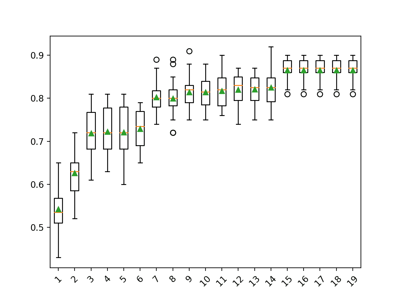
Box Plot of SVD Number of Components vs. Classification Accuracy
We may choose to use an SVD transform and logistic regression model combination as our final model.
This involves fitting the Pipeline on all available data and using the pipeline to make predictions on new data. Importantly, the same transform must be performed on this new data, which is handled automatically via the Pipeline.
The code below provides an example of fitting and using a final model with SVD transforms on new data.
|
1 2 3 4 5 6 7 8 9 10 11 12 13 14 15 16 |
# make predictions using svd with logistic regression from sklearn.datasets import make_classification from sklearn.pipeline import Pipeline from sklearn.decomposition import TruncatedSVD from sklearn.linear_model import LogisticRegression # define dataset X, y = make_classification(n_samples=1000, n_features=20, n_informative=15, n_redundant=5, random_state=7) # define the model steps = [('svd', TruncatedSVD(n_components=15)), ('m', LogisticRegression())] model = Pipeline(steps=steps) # fit the model on the whole dataset model.fit(X, y) # make a single prediction row = [[0.2929949,-4.21223056,-1.288332,-2.17849815,-0.64527665,2.58097719,0.28422388,-7.1827928,-1.91211104,2.73729512,0.81395695,3.96973717,-2.66939799,3.34692332,4.19791821,0.99990998,-0.30201875,-4.43170633,-2.82646737,0.44916808]] yhat = model.predict(row) print('Predicted Class: %d' % yhat[0]) |
Running the example fits the Pipeline on all available data and makes a prediction on new data.
Here, the transform uses the 15 most important components from the SVD transform, as we found from testing above.
A new row of data with 20 columns is provided and is automatically transformed to 15 components and fed to the logistic regression model in order to predict the class label.
|
1 |
Predicted Class: 1 |
Further Reading
This section provides more resources on the topic if you are looking to go deeper.
Tutorials
- A Gentle Introduction to Sparse Matrices for Machine Learning
- How to Calculate the SVD from Scratch with Python
Papers
Books
- Machine Learning: A Probabilistic Perspective, 2012.
- Data Mining: Practical Machine Learning Tools and Techniques, 4th edition, 2016.
- Pattern Recognition and Machine Learning, 2006.
APIs
- Decomposing signals in components (matrix factorization problems), scikit-learn.
- sklearn.decomposition.TruncatedSVD API.
- sklearn.pipeline.Pipeline API.
Articles
- Dimensionality reduction, Wikipedia.
- Curse of dimensionality, Wikipedia.
- Singular value decomposition, Wikipedia.
Summary
In this tutorial, you discovered how to use SVD for dimensionality reduction when developing predictive models.
Specifically, you learned:
- Dimensionality reduction involves reducing the number of input variables or columns in modeling data.
- SVD is a technique from linear algebra that can be used to automatically perform dimensionality reduction.
- How to evaluate predictive models that use an SVD projection as input and make predictions with new raw data.
Do you have any questions?
Ask your questions in the comments below and I will do my best to answer.
Get a Handle on Modern Data Preparation!

Prepare Your Machine Learning Data in Minutes
...with just a few lines of python code
Discover how in my new Ebook:
Data Preparation for Machine Learning
It provides self-study tutorials with full working code on:
Feature Selection, RFE, Data Cleaning, Data Transforms, Scaling, Dimensionality Reduction,
and much more...


Hi, you mentioned that SVD is typically used on sparse data and PCA is better for dense data. Could you explain why?
From a high-level – because of the nature of each technique.
Hi sorry, do you mind further elaborating?
Sure, you can learn more about how SVD is calculated here:
https://machinelearningmastery.com/singular-value-decomposition-for-machine-learning/
You can learn more about how PCA is calculated here:
https://machinelearningmastery.com/calculate-principal-component-analysis-scratch-python/
You could have used a Naive Bayes model,to compare the accuracy with the LDA example.
Sorry, I don’t follow. What do you mean?
In the tutorial about LDA you used the Naive Bayes model and got an accuracy of 0.3. I just got curious If the svd with Bayes here would have the same accuracy of 0.8 that you got.
Ah I see.
I guess we are not trying to get the best performance, but instead demonstrate how to use the method so that you can copy-paste it and use it on your own project.
You meantion: “In essence, the original features no longer exist and new features are constructed from the available data that are not directly comparable to the original data, e.g. don’t have column names.”
But what if I want to go back to the original feature space in an approximate sense?
Say I after classification using the datapoints in reduced space, I find that 2nd, 3rd and 6th component are highest ranked in terms of some importance metric. Now I want to go back to original feature space and find out what combination of the original features is component #2.
How do I do that?
Good question, you can see the calculation here:
https://machinelearningmastery.com/singular-value-decomposition-for-machine-learning/
Try playing with the example and different reconstructions.
can we use this for mixed data type?
The example is for numeric data.
There may be an extension for ordinal/categorical variables. I’m not across it, sorry.
Hi,
Can we apply SVD for dimensionality reduction when the number of samples are less than the number of features?
I am trying to find the way that i can reduce the dimension of that kind of data..
Yes, I believe so.
What is the range of values after applying truncated svd and what these values reflect ??
If you have a NxD matrix as input, representing N data points, each in D dimensions, then after applying TruncatedSVD with default (n_components=2), then you get a Nx2 matrix of the same N data points but only in 2 dimensions. This is a reduced dimension that allows you to use a simpler model.
Hi, can you provide any content that describes in more detail the process of performing SVD on new data, based on the SVD fit?
I’m having trouble understanding how the SVD is saved in the pipeline, and if so, what values are required to perform the fitted SVD on new data.
I apologize if the question is not entirely clear.
Hi Al…the following may help clarify:
https://www.analyticsvidhya.com/blog/2019/08/5-applications-singular-value-decomposition-svd-data-science/
Hi James,
Thanks for the response. I took a look through the article you shared. It does a great job of explaining the basics of SVD and it’s applications, but I couldn’t find exactly what I’m trying to understand.
I will try to illustrate below my confusion. I followed the steps laid out here: https://machinelearningmastery.com/singular-value-decomposition-for-machine-learning/
To start I will create a Matrix A and perform truncated SVD with n_components = 2…
A = array([
[1,2,3,4,5,6,7,8,9,10],
[11,12,13,14,15,16,17,18,19,20],
[21,22,23,24,25,26,27,28,29,30]])
truncatedA = array([
[-18.52157747 6.47697214]
[-49.81310011 1.91182038]
[-81.10462276 -2.65333138]])
Next I will pretend that in the future we will receive a new data point that matches identically the first row of Matrix A
new_data = array([
[1,2,3,4,5,6,7,8,9,10]])
When I use the truncatedSVD method on this new matrix, the result is as follows:
new_truncated = array([
[[-1.96214169e+01 -1.11022302e-16]])
So I think that this is where my understanding of the subject is lacking. I would have expected that the first row of the first truncated result would match the second truncated result.
Hi James,
Clearly I still have a bunch of reading to do, but I was able to figure out my problem by playing through my python code.
The following works:
Perform SVD on training set, save the VT.T
Then when I receive new data, I simply take the dot product of saved VT.T and the new data array.