Datasets may have missing values, and this can cause problems for many machine learning algorithms.
As such, it is good practice to identify and replace missing values for each column in your input data prior to modeling your prediction task. This is called missing data imputation, or imputing for short.
A sophisticated approach involves defining a model to predict each missing feature as a function of all other features and to repeat this process of estimating feature values multiple times. The repetition allows the refined estimated values for other features to be used as input in subsequent iterations of predicting missing values. This is generally referred to as iterative imputation.
In this tutorial, you will discover how to use iterative imputation strategies for missing data in machine learning.
After completing this tutorial, you will know:
Missing values must be marked with NaN values and can be replaced with iteratively estimated values.
How to load a CSV value with missing values and mark the missing values with NaN values and report the number and percentage of missing values for each column.
How to impute missing values with iterative models as a data preparation method when evaluating models and when fitting a final model to make predictions on new data.
Kick-start your project with my new book Data Preparation for Machine Learning, including step-by-step tutorials and the Python source code files for all examples.
Let’s get started.
Updated Jun/2020: Changed the column used for prediction in examples.
Iterative Imputation for Missing Values in Machine Learning Photo by Gergely Csatari, some rights reserved.
Tutorial Overview
This tutorial is divided into three parts; they are:
Iterative Imputation
Horse Colic Dataset
Iterative Imputation With IterativeImputer
IterativeImputer Data Transform
IterativeImputer and Model Evaluation
IterativeImputer and Different Imputation Order
IterativeImputer and Different Number of Iterations
IterativeImputer Transform When Making a Prediction
Iterative Imputation
A dataset may have missing values.
These are rows of data where one or more values or columns in that row are not present. The values may be missing completely or they may be marked with a special character or value, such as a question mark “?”.
Values could be missing for many reasons, often specific to the problem domain, and might include reasons such as corrupt measurements or unavailability.
Most machine learning algorithms require numeric input values, and a value to be present for each row and column in a dataset. As such, missing values can cause problems for machine learning algorithms.
As such, it is common to identify missing values in a dataset and replace them with a numeric value. This is called data imputing, or missing data imputation.
One approach to imputing missing values is to use an iterative imputation model.
Iterative imputation refers to a process where each feature is modeled as a function of the other features, e.g. a regression problem where missing values are predicted. Each feature is imputed sequentially, one after the other, allowing prior imputed values to be used as part of a model in predicting subsequent features.
It is iterative because this process is repeated multiple times, allowing ever improved estimates of missing values to be calculated as missing values across all features are estimated.
This approach may be generally referred to as fully conditional specification (FCS) or multivariate imputation by chained equations (MICE).
This methodology is attractive if the multivariate distribution is a reasonable description of the data. FCS specifies the multivariate imputation model on a variable-by-variable basis by a set of conditional densities, one for each incomplete variable. Starting from an initial imputation, FCS draws imputations by iterating over the conditional densities. A low number of iterations (say 10–20) is often sufficient.
Different regression algorithms can be used to estimate the missing values for each feature, although linear methods are often used for simplicity. The number of iterations of the procedure is often kept small, such as 10. Finally, the order that features are processed sequentially can be considered, such as from the feature with the least missing values to the feature with the most missing values.
Now that we are familiar with iterative methods for missing value imputation, let’s take a look at a dataset with missing values.
Want to Get Started With Data Preparation?
Take my free 7-day email crash course now (with sample code).
Click to sign-up and also get a free PDF Ebook version of the course.
Horse Colic Dataset
The horse colic dataset describes medical characteristics of horses with colic and whether they lived or died.
There are 300 rows and 26 input variables with one output variable. It is a binary classification prediction task that involves predicting 1 if the horse lived and 2 if the horse died.
There are many fields we could select to predict in this dataset. In this case, we will predict whether the problem was surgical or not (column index 23), making it a binary classification problem.
The dataset has many missing values for many of the columns where each missing value is marked with a question mark character (“?”).
Below provides an example of rows from the dataset with marked missing values.
4 2.0 1 530255 37.3 104.0 35.0 NaN ... NaN 2.0 2 4300 0 0 2
[5 rows x 28 columns]
Next, we can see the list of all columns in the dataset and the number and percentage of missing values.
We can see that some columns (e.g. column indexes 1 and 2) have no missing values and other columns (e.g. column indexes 15 and 21) have many or even a majority of missing values.
1
2
3
4
5
6
7
8
9
10
11
12
13
14
15
16
17
18
19
20
21
22
23
24
25
26
27
28
> 0, Missing: 1 (0.3%)
> 1, Missing: 0 (0.0%)
> 2, Missing: 0 (0.0%)
> 3, Missing: 60 (20.0%)
> 4, Missing: 24 (8.0%)
> 5, Missing: 58 (19.3%)
> 6, Missing: 56 (18.7%)
> 7, Missing: 69 (23.0%)
> 8, Missing: 47 (15.7%)
> 9, Missing: 32 (10.7%)
> 10, Missing: 55 (18.3%)
> 11, Missing: 44 (14.7%)
> 12, Missing: 56 (18.7%)
> 13, Missing: 104 (34.7%)
> 14, Missing: 106 (35.3%)
> 15, Missing: 247 (82.3%)
> 16, Missing: 102 (34.0%)
> 17, Missing: 118 (39.3%)
> 18, Missing: 29 (9.7%)
> 19, Missing: 33 (11.0%)
> 20, Missing: 165 (55.0%)
> 21, Missing: 198 (66.0%)
> 22, Missing: 1 (0.3%)
> 23, Missing: 0 (0.0%)
> 24, Missing: 0 (0.0%)
> 25, Missing: 0 (0.0%)
> 26, Missing: 0 (0.0%)
> 27, Missing: 0 (0.0%)
Now that we are familiar with the horse colic dataset that has missing values, let’s look at how we can use iterative imputation.
Iterative Imputation With IterativeImputer
The scikit-learn machine learning library provides the IterativeImputer class that supports iterative imputation.
In this section, we will explore how to effectively use the IterativeImputer class.
IterativeImputer Data Transform
It is a data transform that is first configured based on the method used to estimate the missing values. By default, a BayesianRidge model is employed that uses a function of all other input features. Features are filled in ascending order, from those with the fewest missing values to those with the most.
The fit imputer is then applied to a dataset to create a copy of the dataset with all missing values for each column replaced with an estimated value.
1
2
3
...
# transform the dataset
Xtrans=imputer.transform(X)
The IterativeImputer class cannot be used directly because it is experimental.
If you try to use it directly, you will get an error as follows:
1
ImportError: cannot import name 'IterativeImputer'
Instead, you must add an additional import statement to add support for the IterativeImputer class, as follows:
1
2
...
from sklearn.experimental import enable_iterative_imputer
We can demonstrate its usage on the horse colic dataset and confirm it works by summarizing the total number of missing values in the dataset before and after the transform.
The complete example is listed below.
1
2
3
4
5
6
7
8
9
10
11
12
13
14
15
16
17
18
19
20
21
22
# iterative imputation transform for the horse colic dataset
from numpy import isnan
from pandas import read_csv
from sklearn.experimental import enable_iterative_imputer
Running the example first loads the dataset and reports the total number of missing values in the dataset as 1,605.
The transform is configured, fit, and performed and the resulting new dataset has no missing values, confirming it was performed as we expected.
Each missing value was replaced with a value estimated by the model.
1
2
Missing: 1605
Missing: 0
IterativeImputer and Model Evaluation
It is a good practice to evaluate machine learning models on a dataset using k-fold cross-validation.
To correctly apply iterative missing data imputation and avoid data leakage, it is required that the models for each column are calculated on the training dataset only, then applied to the train and test sets for each fold in the dataset.
This can be achieved by creating a modeling pipeline where the first step is the iterative imputation, then the second step is the model. This can be achieved using the Pipeline class.
For example, the Pipeline below uses an IterativeImputer with the default strategy, followed by a random forest model.
Running the example correctly applies data imputation to each fold of the cross-validation procedure.
Note: Your results may vary given the stochastic nature of the algorithm or evaluation procedure, or differences in numerical precision. Consider running the example a few times and compare the average outcome.
The pipeline is evaluated using three repeats of 10-fold cross-validation and reports the mean classification accuracy on the dataset as about 86.3 percent which is a good score.
1
Mean Accuracy: 0.863 (0.057)
How do we know that using a default iterative strategy is good or best for this dataset?
The answer is that we don’t.
IterativeImputer and Different Imputation Order
By default, imputation is performed in ascending order from the feature with the least missing values to the feature with the most.
This makes sense as we want to have more complete data when it comes time to estimating missing values for columns where the majority of values are missing.
Nevertheless, we can experiment with different imputation order strategies, such as descending, right-to-left (Arabic), left-to-right (Roman), and random.
The example below evaluates and compares each available imputation order configuration.
1
2
3
4
5
6
7
8
9
10
11
12
13
14
15
16
17
18
19
20
21
22
23
24
25
26
27
28
29
30
31
32
33
34
# compare iterative imputation strategies for the horse colic dataset
from numpy import mean
from numpy import std
from pandas import read_csv
from sklearn.ensemble import RandomForestClassifier
from sklearn.experimental import enable_iterative_imputer
from sklearn.impute import IterativeImputer
from sklearn.model_selection import cross_val_score
from sklearn.model_selection import RepeatedStratifiedKFold
Running the example evaluates each imputation order on the horse colic dataset using repeated cross-validation.
Note: Your results may vary given the stochastic nature of the algorithm or evaluation procedure, or differences in numerical precision. Consider running the example a few times and compare the average outcome.
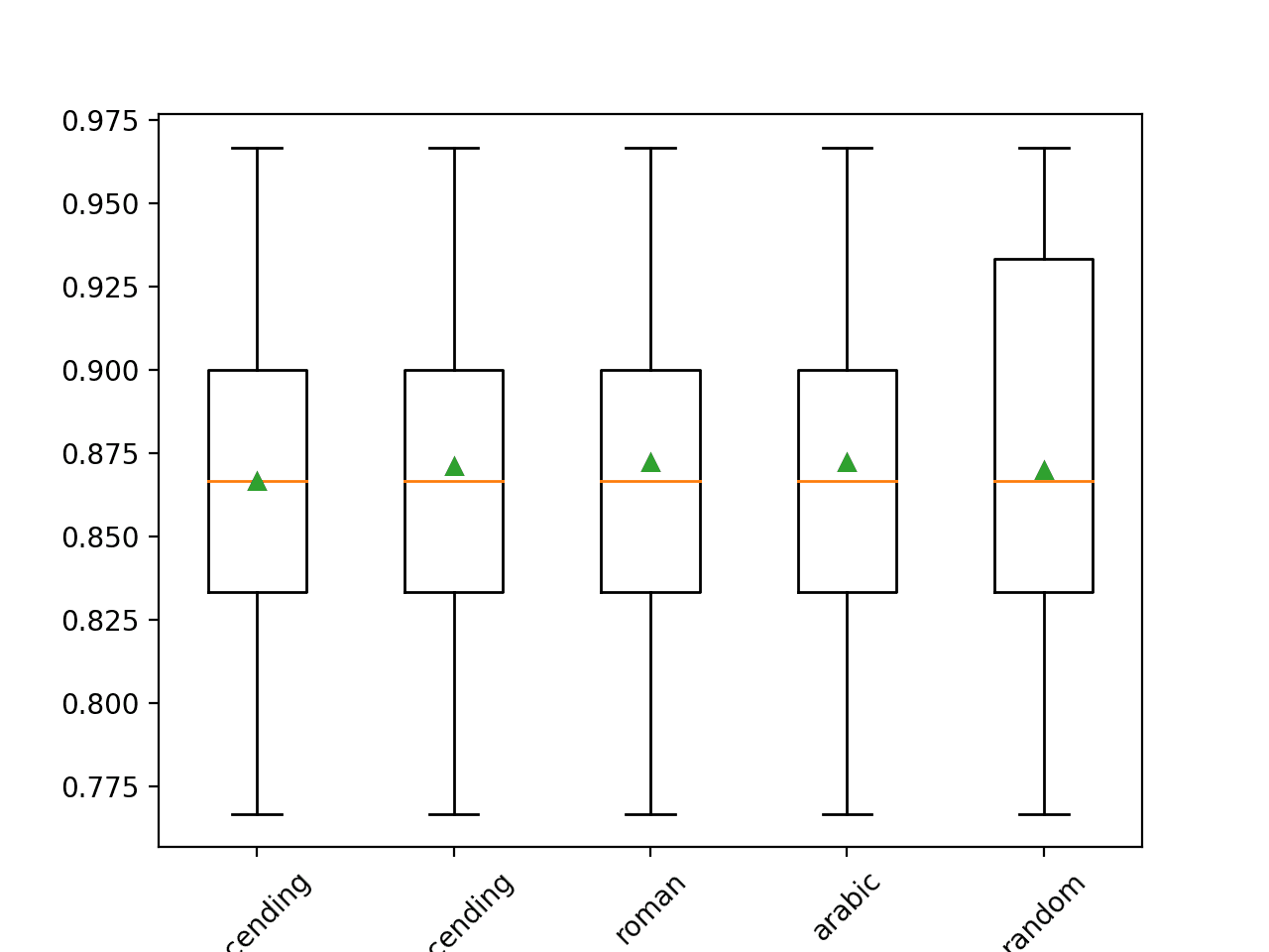
The mean accuracy of each strategy is reported along the way. The results suggest little difference between most of the methods, with descending (opposite of the default) performing the best. The results suggest that Arabic (right-to-left) or Roman order might be better for this dataset with an accuracy of about 87.2 percent.
1
2
3
4
5
>ascending 0.867 (0.049)
>descending 0.871 (0.052)
>roman 0.872 (0.052)
>arabic 0.872 (0.052)
>random 0.870 (0.060)
At the end of the run, a box and whisker plot is created for each set of results, allowing the distribution of results to be compared.
Box and Whisker Plot of Imputation Order Strategies Applied to the Horse Colic Dataset
IterativeImputer and Different Number of Iterations
By default, the IterativeImputer will repeat the number of iterations 10 times.
It is possible that a large number of iterations may begin to bias or skew the estimate and that few iterations may be preferred. The number of iterations of the procedure can be specified via the “max_iter” argument.
It may be interesting to evaluate different numbers of iterations. The example below compares different values for “max_iter” from 1 to 20.
1
2
3
4
5
6
7
8
9
10
11
12
13
14
15
16
17
18
19
20
21
22
23
24
25
26
27
28
29
30
31
32
33
34
# compare iterative imputation number of iterations for the horse colic dataset
from numpy import mean
from numpy import std
from pandas import read_csv
from sklearn.ensemble import RandomForestClassifier
from sklearn.experimental import enable_iterative_imputer
from sklearn.impute import IterativeImputer
from sklearn.model_selection import cross_val_score
from sklearn.model_selection import RepeatedStratifiedKFold
Running the example evaluates each number of iterations on the horse colic dataset using repeated cross-validation.
Note: Your results may vary given the stochastic nature of the algorithm or evaluation procedure, or differences in numerical precision. Consider running the example a few times and compare the average outcome.
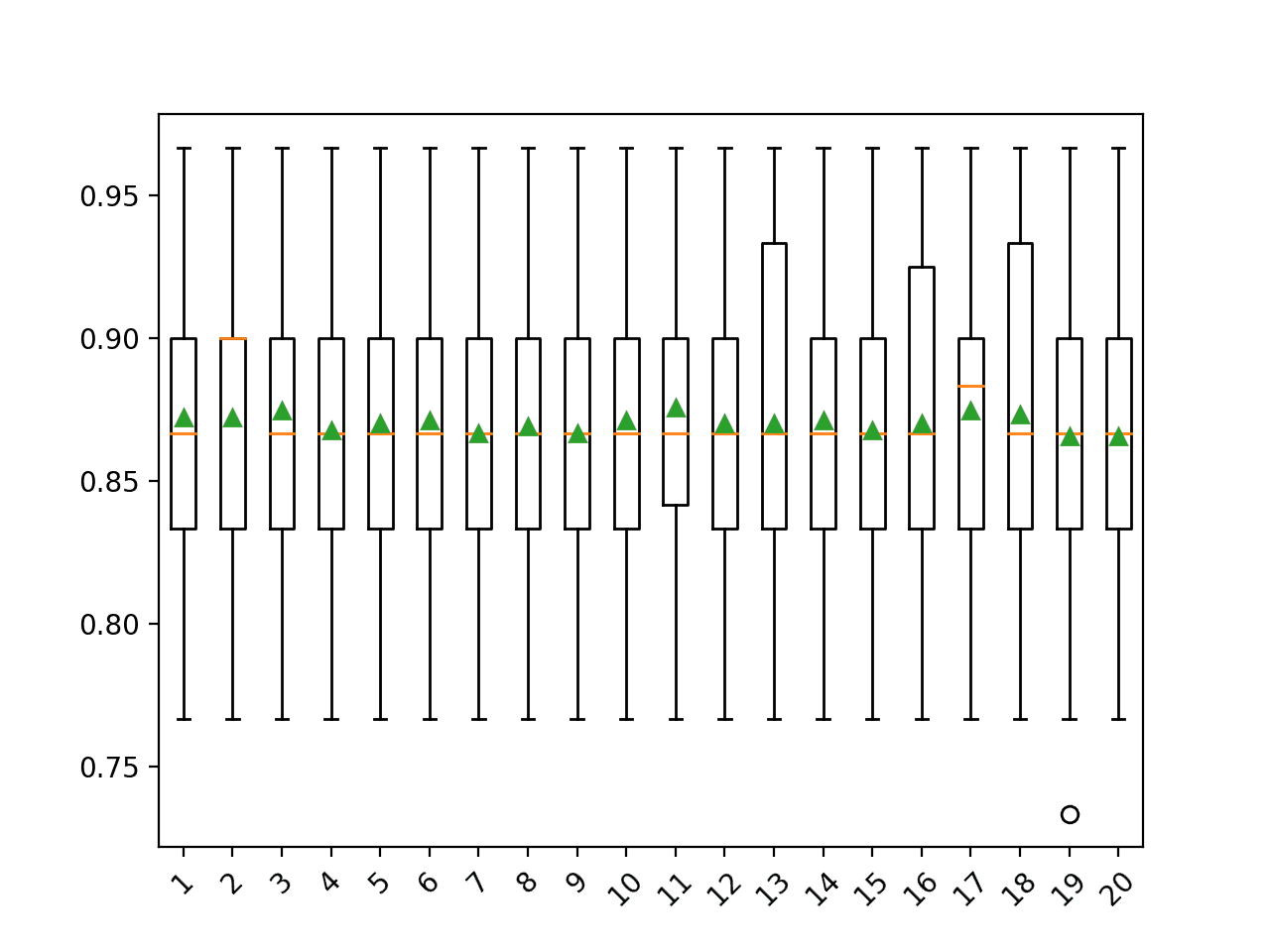
The results suggest that very few iterations, such as 3, might be as or more effective than 9-12 iterations on this dataset.
1
2
3
4
5
6
7
8
9
10
11
12
13
14
15
16
17
18
19
20
>1 0.872 (0.053)
>2 0.872 (0.052)
>3 0.874 (0.051)
>4 0.868 (0.050)
>5 0.870 (0.050)
>6 0.871 (0.051)
>7 0.867 (0.055)
>8 0.869 (0.054)
>9 0.867 (0.054)
>10 0.871 (0.051)
>11 0.876 (0.047)
>12 0.870 (0.053)
>13 0.870 (0.056)
>14 0.871 (0.053)
>15 0.868 (0.057)
>16 0.870 (0.053)
>17 0.874 (0.051)
>18 0.873 (0.054)
>19 0.866 (0.054)
>20 0.866 (0.051)
At the end of the run, a box and whisker plot is created for each set of results, allowing the distribution of results to be compared.
Box and Whisker Plot of Number of Imputation Iterations on the Horse Colic Dataset
IterativeImputer Transform When Making a Prediction
We may wish to create a final modeling pipeline with the iterative imputation and random forest algorithm, then make a prediction for new data.
This can be achieved by defining the pipeline and fitting it on all available data, then calling the predict() function, passing new data in as an argument.
Importantly, the row of new data must mark any missing values using the NaN value.
In this tutorial, you discovered how to use iterative imputation strategies for missing data in machine learning.
Specifically, you learned:
Missing values must be marked with NaN values and can be replaced with iteratively estimated values.
How to load a CSV value with missing values and mark the missing values with NaN values and report the number and percentage of missing values for each column.
How to impute missing values with iterative models as a data preparation method when evaluating models and when fitting a final model to make predictions on new data.
Do you have any questions?
Ask your questions in the comments below and I will do my best to answer.
It provides self-study tutorials with full working code on: Feature Selection, RFE, Data Cleaning, Data Transforms, Scaling, Dimensionality Reduction,
and much more...
Bring Modern Data Preparation Techniques to Your Machine Learning Projects
Hello Jason,
I’ve a question about linear regression.
Is there any way to tackle linear regression step by step: i.e is there a flow
to adress a linear regression problem (from where I have to start to an and).
Do you have an easy example of linear regression?
Thanks,
Marco
Learned a new data imputation technique through this article. Thanks a lot Jason. Earlier I only used to replace the missing values with the mean or median of the available values. Will definitely apply this technique in my upcoming project.
Thank you for your tutorial on IterativeImputer, I’ve learned a lot from this post.
I’ve a question on the missing value topic: does it generally (for most cases maybe) perform better if we use IterativeImputer instead of mode or mean to fill the missing value ?
I tried the horse_colic dataset, but in my case, mode and mean work better than IterativeImputer. Nevertheless, I’ve seen many posts of choosing IterativeImputer as the default tool to deal with missing values. I thought people are using it must because it works better.
Thanks Jason. Enlightening as always. My take-away on this is that by imputing missing values, you get to keep the row for training, thus strengthening the signal from the values that were originally present. Should your goal of imputation be to create values that have a neutral contribution to training those associated parameters? Otherwise it seems you run the risk of overfitting. I suppose the validation metrics are the best measure of whether you chose the correct method of imputation. And as you’ve engrained into me from your other articles and confirmed in your examples above, imputation gets applied “inside the fold.”
Jason, thanks a lot for that useful guide! But I have a question. Is it better to apply scaling before the missing data imputation? To estimate the NaNs the linear regression methods are used, which prefer scaled data.
Hi Jason,
I learned so much reading your articles. I tried this on the ‘informal polling questions’ dataset. Dataset is having so many missing values. I have applied both KNN imputation and Iterative imputation in filling the missing values. but I am getting only 68 % accuracy can apply a classification algorithm to predict the accuracy of test data?
I’m curious, and I can’t seem to find any documentation. What does the iterative imputer do if it encounters a row that is completely missing – every value is nan?
Thank you for this tutorial. I am trying this iterative imputer over integer data, but I am getting error like “ufunc ‘isnan’ not supported for the input types, and the inputs could not be safely coerced to any supported types according to the casting rule ”safe””. How could I correct this? My guess is I need to change the dtype! Cannot figure out how to do it.
Thank you for this tutorial.
But I have a question
if there are the missing values in category column such like ” Job” and the values is 1~6 represent different level of the jobs . How can I use the model ? Can I use linear model ?
second . If the missing value in each column is almost 40% … but I think that’s important and I can’t drop it . is there any helpful way I can use ?
the data is time series data but the missing value are all in the category columns such like person’s age ,zip code,income level 、Job level .
I was working with this IterativeImputer and I have some questions.
If I encode the categorical variables with OneHotEncoder, the imputer.fit() gives an error “setting an array element with a sequence”, what could be the possible solution?
When there is no response variable, the goal is just to impute the missing values (not predict anything), is there any way to measure how well IterativeImputer is performing to impute the missing values?
Again, thank you for the tutorial. It helped a lot to figure out the process.
Hi Jason, thank you. Your suggestion worked. Now I have another question. It would great to have your suggestion.
When I am imputing categorical variables (after encoding them), the data type changes from object to float. To find the accuracy after imputation, I am rounding them so that I can compare them with the encoded labels. Am I missing something here? Or all datatypes are converted to float after imputation with iterative imputer?
Please note, I am not doing any kind of prediction, just imputing the missing values. So there is no Y variable. Also, the dataset does not have any missing values. I have added the missing values by randomly deleting some cell values so that I can compute the accuracy after imputation.
According to the sklearn.impute.IterativeImputer user guide, the estimator parameter can be a different kind of regression algorithm such as BayesianRidge ,DecisionTreeRegressor, and so on. My question is that can we use a classification algorithm such as SVC, KNN classifier instead of regression as an estimator parameter?
Another great tutorial! Thanks Jason! I just want to ask though. when and how do we decide on what estimator to put inside IterativeImputer()? Is the default estimator (BayesianRidge()) often used?
Thanks for the great read. I learned a lot. Traditionally, I’ve ran my RF pipeline using sklearn’s train_test_split function, which I don’t see here as you’re later using k-fold CV. My understanding is that imputation should be done separately on the training and testing data – is that correct? Is there a simple way to go about this?
Thanks a lot for this step by step tutorial, it is very well explained and detail, thank you so much.
In the Iterative Imputation With IterativeImputer paragraph, where does the value “23” comes from?
# split into input and output elements
data = dataframe.values
ix = [i for i in range(data.shape[1]) if i != 23]
X, y = data[:, ix], data[:, 23]
Also, the dataframe originally contains 28 columns but the array Xtrans only contains 27 lists (or 27 columns once converted to a DataFrame) so did I miss something or did we lose 1 column on the way?
Thanks a lot for your feedback and have a nice day.
I tried using IterativeImputer compare to R’s MICE, I found one interesting, but disturbing result. When I predicted the imputed test set, the AUC was significantly higher (0.85 vs 0.81) than predicted only complete case analysis (around 50% of rows).
I tried to look for the data leakage, I split the test set out before imputing and use transform on the test set, of course without target variable inside the imputing dataframe.
This problem was not happenning with R’s MICE, the AUC of the imputed test set and complete case analysis were roughly the same.
1. How do we use Iterative Imputer when we have missing value in for categorical and numerical columns
1.1. Should we impute values separately ?
1.2 How do we select which feature to use for imputation in each case?
Iterative imputer will replace column headings in a dataframe, watch out for this. It does it during the transform step, you need to save col headings and then put them back after the transform


Hi Jason,
You don’t know how much I’ve enjoyed doing this. I’m learning ML and this has added much to my data cleaning knowledge. Asante sana!
Thanks!
Hello Jason,
I’ve a question about linear regression.
Is there any way to tackle linear regression step by step: i.e is there a flow
to adress a linear regression problem (from where I have to start to an and).
Do you have an easy example of linear regression?
Thanks,
Marco
Yes, this general process:
https://machinelearningmastery.com/start-here/#process
Learned a new data imputation technique through this article. Thanks a lot Jason. Earlier I only used to replace the missing values with the mean or median of the available values. Will definitely apply this technique in my upcoming project.
Thanks, I’m happy to hear that!
Thank you for your tutorial on IterativeImputer, I’ve learned a lot from this post.
I’ve a question on the missing value topic: does it generally (for most cases maybe) perform better if we use IterativeImputer instead of mode or mean to fill the missing value ?
I tried the horse_colic dataset, but in my case,
modeandmeanwork better thanIterativeImputer. Nevertheless, I’ve seen many posts of choosingIterativeImputeras the default tool to deal with missing values. I thought people are using it must because it works better.In case you’re interested, I tried
xgbooston this dataset. WithIterativeImputerI got an accuracy score0.831(0.048), and0.848 (0.061)withmean.python
model = xgboost.XGBClassifier()
imputer = IterativeImputer()
pipeline = Pipeline(steps=[('i', imputer), ('m', model)])
cv = RepeatedStratifiedKFold(n_splits=10, n_repeats=3, random_state=0)
Nice work!
You’re welcome.
It depends on the dataset and the model. Try a range of methods and discover what works best for your dataset.
Thanks Jason. Enlightening as always. My take-away on this is that by imputing missing values, you get to keep the row for training, thus strengthening the signal from the values that were originally present. Should your goal of imputation be to create values that have a neutral contribution to training those associated parameters? Otherwise it seems you run the risk of overfitting. I suppose the validation metrics are the best measure of whether you chose the correct method of imputation. And as you’ve engrained into me from your other articles and confirmed in your examples above, imputation gets applied “inside the fold.”
Yes, you want to test to confirm that it adds benefit to your prediction task.
It can help with training, but also test data, and new data for which a prediction is required.
Yes, always within the fold to avoid data leakage and an optimistic estimate of model preformance.
Jason, thanks a lot for that useful guide! But I have a question. Is it better to apply scaling before the missing data imputation? To estimate the NaNs the linear regression methods are used, which prefer scaled data.
Probably after.
Thank you for the tutorial, I’ve learned a lot from this post. This is really a very informative article.
I’m happy to hear that.
Hi Jason,
I learned so much reading your articles. I tried this on the ‘informal polling questions’ dataset. Dataset is having so many missing values. I have applied both KNN imputation and Iterative imputation in filling the missing values. but I am getting only 68 % accuracy can apply a classification algorithm to predict the accuracy of test data?
Thanks!
Perhaps try an alternate algorithm or config or data preparation scheme?
I’m curious, and I can’t seem to find any documentation. What does the iterative imputer do if it encounters a row that is completely missing – every value is nan?
Probably nothing or error. In that case, the column should be removed first.
Thank you for this tutorial. I am trying this iterative imputer over integer data, but I am getting error like “ufunc ‘isnan’ not supported for the input types, and the inputs could not be safely coerced to any supported types according to the casting rule ”safe””. How could I correct this? My guess is I need to change the dtype! Cannot figure out how to do it.
Perhaps confirm your libraries are up to date?
Perhaps confirm you don’t have any nan’s in your data?
Thank you for this tutorial.
But I have a question
if there are the missing values in category column such like ” Job” and the values is 1~6 represent different level of the jobs . How can I use the model ? Can I use linear model ?
second . If the missing value in each column is almost 40% … but I think that’s important and I can’t drop it . is there any helpful way I can use ?
the data is time series data but the missing value are all in the category columns such like person’s age ,zip code,income level 、Job level .
please help me thank you !
If you have missing values, perhaps try imputing them with statistics, a knn or iterative imputation.
Compare results to models fit on data with rows or cols with missing values removed.
Thank you for the informative tutorial.
I was working with this IterativeImputer and I have some questions.
If I encode the categorical variables with OneHotEncoder, the imputer.fit() gives an error “setting an array element with a sequence”, what could be the possible solution?
When there is no response variable, the goal is just to impute the missing values (not predict anything), is there any way to measure how well IterativeImputer is performing to impute the missing values?
Again, thank you for the tutorial. It helped a lot to figure out the process.
You’re welcome.
Perhaps use an ordinal encoder and compare the results?
Hi Jason, thank you. Your suggestion worked. Now I have another question. It would great to have your suggestion.
When I am imputing categorical variables (after encoding them), the data type changes from object to float. To find the accuracy after imputation, I am rounding them so that I can compare them with the encoded labels. Am I missing something here? Or all datatypes are converted to float after imputation with iterative imputer?
Please note, I am not doing any kind of prediction, just imputing the missing values. So there is no Y variable. Also, the dataset does not have any missing values. I have added the missing values by randomly deleting some cell values so that I can compute the accuracy after imputation.
You’re welcome.
All input variables in machine learning are float, even integers – at least in Python/sklearn this is the case.
Converting data types into your preferred type after data preparation is a good idea if you’re not modeling.
Hi ,jason
Thank you for the amazing information.
According to the sklearn.impute.IterativeImputer user guide, the estimator parameter can be a different kind of regression algorithm such as BayesianRidge ,DecisionTreeRegressor, and so on. My question is that can we use a classification algorithm such as SVC, KNN classifier instead of regression as an estimator parameter?
Yes, perhaps try it and compare results to see if it makes a big difference on your dataaset.
Another great tutorial! Thanks Jason! I just want to ask though. when and how do we decide on what estimator to put inside IterativeImputer()? Is the default estimator (BayesianRidge()) often used?
Thanks.
Perhaps you can use a little trial and error and discover what works well or best for your dataset.
Hi Jason,
Thanks for the great read. I learned a lot. Traditionally, I’ve ran my RF pipeline using sklearn’s train_test_split function, which I don’t see here as you’re later using k-fold CV. My understanding is that imputation should be done separately on the training and testing data – is that correct? Is there a simple way to go about this?
Thanks!
Yes, imputation would be fit on the training set and applied to the train and test sets, see this
https://machinelearningmastery.com/data-preparation-without-data-leakage/
Hi Jason,
Thanks a lot for this step by step tutorial, it is very well explained and detail, thank you so much.
In the Iterative Imputation With IterativeImputer paragraph, where does the value “23” comes from?
# split into input and output elements
data = dataframe.values
ix = [i for i in range(data.shape[1]) if i != 23]
X, y = data[:, ix], data[:, 23]
Also, the dataframe originally contains 28 columns but the array Xtrans only contains 27 lists (or 27 columns once converted to a DataFrame) so did I miss something or did we lose 1 column on the way?
Thanks a lot for your feedback and have a nice day.
We remove a variable from the dataset that is not useful.
Hi Jason, again, thank you for a great post.
I tried using IterativeImputer compare to R’s MICE, I found one interesting, but disturbing result. When I predicted the imputed test set, the AUC was significantly higher (0.85 vs 0.81) than predicted only complete case analysis (around 50% of rows).
I tried to look for the data leakage, I split the test set out before imputing and use transform on the test set, of course without target variable inside the imputing dataframe.
This problem was not happenning with R’s MICE, the AUC of the imputed test set and complete case analysis were roughly the same.
Thank you
Hi Jason ,
Great article!
I had a few questions:
1. How do we use Iterative Imputer when we have missing value in for categorical and numerical columns
1.1. Should we impute values separately ?
1.2 How do we select which feature to use for imputation in each case?
Hi Bipin…The following is a great starting point to address your questions:
https://scikit-learn.org/stable/modules/impute.html
Iterative imputer will replace column headings in a dataframe, watch out for this. It does it during the transform step, you need to save col headings and then put them back after the transform
Hey can we impute for categorical features?
Hi Ceo…The following may be of interest:
https://www.analyticsvidhya.com/blog/2021/04/how-to-handle-missing-values-of-categorical-variables/