Feature selection is the process of identifying and selecting a subset of input features that are most relevant to the target variable.
Feature selection is often straightforward when working with real-valued input and output data, such as using the Pearson’s correlation coefficient, but can be challenging when working with numerical input data and a categorical target variable.
The two most commonly used feature selection methods for numerical input data when the target variable is categorical (e.g. classification predictive modeling) are the ANOVA f-test statistic and the mutual information statistic.
In this tutorial, you will discover how to perform feature selection with numerical input data for classification.
After completing this tutorial, you will know:
- The diabetes predictive modeling problem with numerical inputs and binary classification target variables.
- How to evaluate the importance of numerical features using the ANOVA f-test and mutual information statistics.
- How to perform feature selection for numerical data when fitting and evaluating a classification model.
Kick-start your project with my new book Data Preparation for Machine Learning, including step-by-step tutorials and the Python source code files for all examples.
Let’s get started.

How to Perform Feature Selection With Numerical Input Data
Photo by Susanne Nilsson, some rights reserved.
Tutorial Overview
This tutorial is divided into four parts; they are:
- Diabetes Numerical Dataset
- Numerical Feature Selection
- ANOVA f-test Feature Selection
- Mutual Information Feature Selection
- Modeling With Selected Features
- Model Built Using All Features
- Model Built Using ANOVA f-test Features
- Model Built Using Mutual Information Features
- Tune the Number of Selected Features
Diabetes Numerical Dataset
As the basis of this tutorial, we will use the so-called “diabetes” dataset that has been widely studied as a machine learning dataset since 1990.
The dataset classifies patients’ data as either an onset of diabetes within five years or not. There are 768 examples and eight input variables. It is a binary classification problem.
A naive model can achieve an accuracy of about 65 percent on this dataset. A good score is about 77 percent +/- 5 percent. We will aim for this region but note that the models in this tutorial are not optimized; they are designed to demonstrate feature selection schemes.
You can download the dataset and save the file as “pima-indians-diabetes.csv” in your current working directory.
- Diabetes Dataset (pima-indians-diabetes.csv)
- Diabetes Dataset Description (pima-indians-diabetes.names)
Looking at the data, we can see that all nine input variables are numerical.
|
1 2 3 4 5 6 |
6,148,72,35,0,33.6,0.627,50,1 1,85,66,29,0,26.6,0.351,31,0 8,183,64,0,0,23.3,0.672,32,1 1,89,66,23,94,28.1,0.167,21,0 0,137,40,35,168,43.1,2.288,33,1 ... |
We can load this dataset into memory using the Pandas library.
|
1 2 3 4 5 |
... # load the dataset as a pandas DataFrame data = read_csv(filename, header=None) # retrieve numpy array dataset = data.values |
Once loaded, we can split the columns into input (X) and output (y) for modeling.
|
1 2 3 4 |
... # split into input (X) and output (y) variables X = dataset[:, :-1] y = dataset[:,-1] |
We can tie all of this together into a helpful function that we can reuse later.
|
1 2 3 4 5 6 7 8 9 10 |
# load the dataset def load_dataset(filename): # load the dataset as a pandas DataFrame data = read_csv(filename, header=None) # retrieve numpy array dataset = data.values # split into input (X) and output (y) variables X = dataset[:, :-1] y = dataset[:,-1] return X, y |
Once loaded, we can split the data into training and test sets so we can fit and evaluate a learning model.
We will use the train_test_split() function form scikit-learn and use 67 percent of the data for training and 33 percent for testing.
|
1 2 3 4 5 |
... # load the dataset X, y = load_dataset('pima-indians-diabetes.csv') # split into train and test sets X_train, X_test, y_train, y_test = train_test_split(X, y, test_size=0.33, random_state=1) |
Tying all of these elements together, the complete example of loading, splitting, and summarizing the raw categorical dataset is listed below.
|
1 2 3 4 5 6 7 8 9 10 11 12 13 14 15 16 17 18 19 20 21 22 |
# load and summarize the dataset from pandas import read_csv from sklearn.model_selection import train_test_split # load the dataset def load_dataset(filename): # load the dataset as a pandas DataFrame data = read_csv(filename, header=None) # retrieve numpy array dataset = data.values # split into input (X) and output (y) variables X = dataset[:, :-1] y = dataset[:,-1] return X, y # load the dataset X, y = load_dataset('pima-indians-diabetes.csv') # split into train and test sets X_train, X_test, y_train, y_test = train_test_split(X, y, test_size=0.33, random_state=1) # summarize print('Train', X_train.shape, y_train.shape) print('Test', X_test.shape, y_test.shape) |
Running the example reports the size of the input and output elements of the train and test sets.
We can see that we have 514 examples for training and 254 for testing.
|
1 2 |
Train (514, 8) (514, 1) Test (254, 8) (254, 1) |
Now that we have loaded and prepared the diabetes dataset, we can explore feature selection.
Want to Get Started With Data Preparation?
Take my free 7-day email crash course now (with sample code).
Click to sign-up and also get a free PDF Ebook version of the course.
Numerical Feature Selection
There are two popular feature selection techniques that can be used for numerical input data and a categorical (class) target variable.
They are:
- ANOVA-f Statistic.
- Mutual Information Statistics.
Let’s take a closer look at each in turn.
ANOVA f-test Feature Selection
ANOVA is an acronym for “analysis of variance” and is a parametric statistical hypothesis test for determining whether the means from two or more samples of data (often three or more) come from the same distribution or not.
An F-statistic, or F-test, is a class of statistical tests that calculate the ratio between variances values, such as the variance from two different samples or the explained and unexplained variance by a statistical test, like ANOVA. The ANOVA method is a type of F-statistic referred to here as an ANOVA f-test.
Importantly, ANOVA is used when one variable is numeric and one is categorical, such as numerical input variables and a classification target variable in a classification task.
The results of this test can be used for feature selection where those features that are independent of the target variable can be removed from the dataset.
When the outcome is numeric, and […] the predictor has more than two levels, the traditional ANOVA F-statistic can be calculated.
— Page 242, Feature Engineering and Selection, 2019.
The scikit-learn machine library provides an implementation of the ANOVA f-test in the f_classif() function. This function can be used in a feature selection strategy, such as selecting the top k most relevant features (largest values) via the SelectKBest class.
For example, we can define the SelectKBest class to use the f_classif() function and select all features, then transform the train and test sets.
|
1 2 3 4 5 6 7 8 9 |
... # configure to select all features fs = SelectKBest(score_func=f_classif, k='all') # learn relationship from training data fs.fit(X_train, y_train) # transform train input data X_train_fs = fs.transform(X_train) # transform test input data X_test_fs = fs.transform(X_test) |
We can then print the scores for each variable (larger is better) and plot the scores for each variable as a bar graph to get an idea of how many features we should select.
|
1 2 3 4 5 6 7 |
... # what are scores for the features for i in range(len(fs.scores_)): print('Feature %d: %f' % (i, fs.scores_[i])) # plot the scores pyplot.bar([i for i in range(len(fs.scores_))], fs.scores_) pyplot.show() |
Tying this together with the data preparation for the diabetes dataset in the previous section, the complete example is listed below.
|
1 2 3 4 5 6 7 8 9 10 11 12 13 14 15 16 17 18 19 20 21 22 23 24 25 26 27 28 29 30 31 32 33 34 35 36 37 38 39 40 41 42 |
# example of anova f-test feature selection for numerical data from pandas import read_csv from sklearn.model_selection import train_test_split from sklearn.feature_selection import SelectKBest from sklearn.feature_selection import f_classif from matplotlib import pyplot # load the dataset def load_dataset(filename): # load the dataset as a pandas DataFrame data = read_csv(filename, header=None) # retrieve numpy array dataset = data.values # split into input (X) and output (y) variables X = dataset[:, :-1] y = dataset[:,-1] return X, y # feature selection def select_features(X_train, y_train, X_test): # configure to select all features fs = SelectKBest(score_func=f_classif, k='all') # learn relationship from training data fs.fit(X_train, y_train) # transform train input data X_train_fs = fs.transform(X_train) # transform test input data X_test_fs = fs.transform(X_test) return X_train_fs, X_test_fs, fs # load the dataset X, y = load_dataset('pima-indians-diabetes.csv') # split into train and test sets X_train, X_test, y_train, y_test = train_test_split(X, y, test_size=0.33, random_state=1) # feature selection X_train_fs, X_test_fs, fs = select_features(X_train, y_train, X_test) # what are scores for the features for i in range(len(fs.scores_)): print('Feature %d: %f' % (i, fs.scores_[i])) # plot the scores pyplot.bar([i for i in range(len(fs.scores_))], fs.scores_) pyplot.show() |
Running the example first prints the scores calculated for each input feature and the target variable.
Note: Your results may vary given the stochastic nature of the algorithm or evaluation procedure, or differences in numerical precision. Consider running the example a few times and compare the average outcome.
In this case, we can see that some features stand out as perhaps being more relevant than others, with much larger test statistic values.
Perhaps features 1, 5, and 7 are most relevant.
|
1 2 3 4 5 6 7 8 |
Feature 0: 16.527385 Feature 1: 131.325562 Feature 2: 0.042371 Feature 3: 1.415216 Feature 4: 12.778966 Feature 5: 49.209523 Feature 6: 13.377142 Feature 7: 25.126440 |
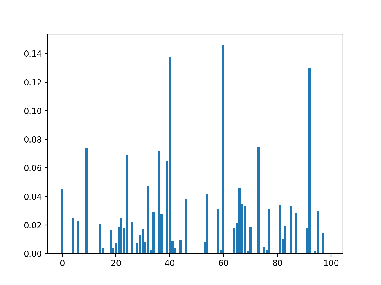
A bar chart of the feature importance scores for each input feature is created.
This clearly shows that feature 1 might be the most relevant (according to test) and that perhaps six of the eight input features are the more relevant.
We could set k=6 when configuring the SelectKBest to select these top four features.
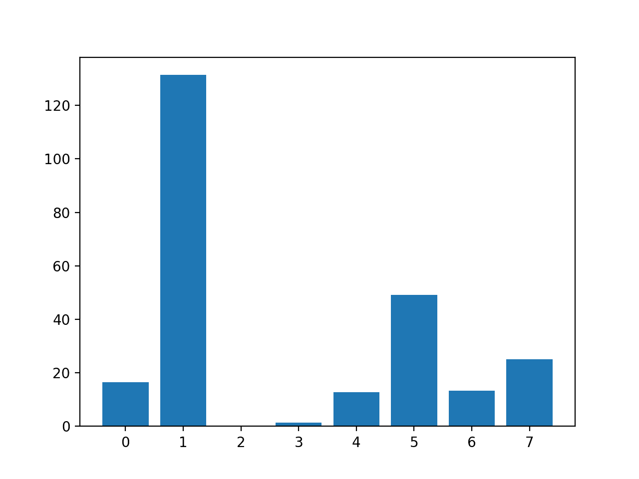
Bar Chart of the Input Features (x) vs The ANOVA f-test Feature Importance (y)
Mutual Information Feature Selection
Mutual information from the field of information theory is the application of information gain (typically used in the construction of decision trees) to feature selection.
Mutual information is calculated between two variables and measures the reduction in uncertainty for one variable given a known value of the other variable.
You can learn more about mutual information in the following tutorial.
Mutual information is straightforward when considering the distribution of two discrete (categorical or ordinal) variables, such as categorical input and categorical output data. Nevertheless, it can be adapted for use with numerical input and categorical output.
For technical details on how this can be achieved, see the 2014 paper titled “Mutual Information between Discrete and Continuous Data Sets.”
The scikit-learn machine learning library provides an implementation of mutual information for feature selection with numeric input and categorical output variables via the mutual_info_classif() function.
Like f_classif(), it can be used in the SelectKBest feature selection strategy (and other strategies).
|
1 2 3 4 5 6 7 8 9 |
... # configure to select all features fs = SelectKBest(score_func=mutual_info_classif, k='all') # learn relationship from training data fs.fit(X_train, y_train) # transform train input data X_train_fs = fs.transform(X_train) # transform test input data X_test_fs = fs.transform(X_test) |
We can perform feature selection using mutual information on the diabetes dataset and print and plot the scores (larger is better) as we did in the previous section.
The complete example of using mutual information for numerical feature selection is listed below.
|
1 2 3 4 5 6 7 8 9 10 11 12 13 14 15 16 17 18 19 20 21 22 23 24 25 26 27 28 29 30 31 32 33 34 35 36 37 38 39 40 41 42 |
# example of mutual information feature selection for numerical input data from pandas import read_csv from sklearn.model_selection import train_test_split from sklearn.feature_selection import SelectKBest from sklearn.feature_selection import mutual_info_classif from matplotlib import pyplot # load the dataset def load_dataset(filename): # load the dataset as a pandas DataFrame data = read_csv(filename, header=None) # retrieve numpy array dataset = data.values # split into input (X) and output (y) variables X = dataset[:, :-1] y = dataset[:,-1] return X, y # feature selection def select_features(X_train, y_train, X_test): # configure to select all features fs = SelectKBest(score_func=mutual_info_classif, k='all') # learn relationship from training data fs.fit(X_train, y_train) # transform train input data X_train_fs = fs.transform(X_train) # transform test input data X_test_fs = fs.transform(X_test) return X_train_fs, X_test_fs, fs # load the dataset X, y = load_dataset('pima-indians-diabetes.csv') # split into train and test sets X_train, X_test, y_train, y_test = train_test_split(X, y, test_size=0.33, random_state=1) # feature selection X_train_fs, X_test_fs, fs = select_features(X_train, y_train, X_test) # what are scores for the features for i in range(len(fs.scores_)): print('Feature %d: %f' % (i, fs.scores_[i])) # plot the scores pyplot.bar([i for i in range(len(fs.scores_))], fs.scores_) pyplot.show() |
Running the example first prints the scores calculated for each input feature and the target variable.
Note: Your results may vary given the stochastic nature of the algorithm or evaluation procedure, or differences in numerical precision. Consider running the example a few times and compare the average outcome.
In this case, we can see that some of the features have a modestly low score, suggesting that perhaps they can be removed.
Perhaps features 1 and 5 are most relevant.
|
1 2 3 4 5 6 7 |
Feature 1: 0.118431 Feature 2: 0.019966 Feature 3: 0.041791 Feature 4: 0.019858 Feature 5: 0.084719 Feature 6: 0.018079 Feature 7: 0.033098 |
A bar chart of the feature importance scores for each input feature is created.
Importantly, a different mixture of features is promoted.
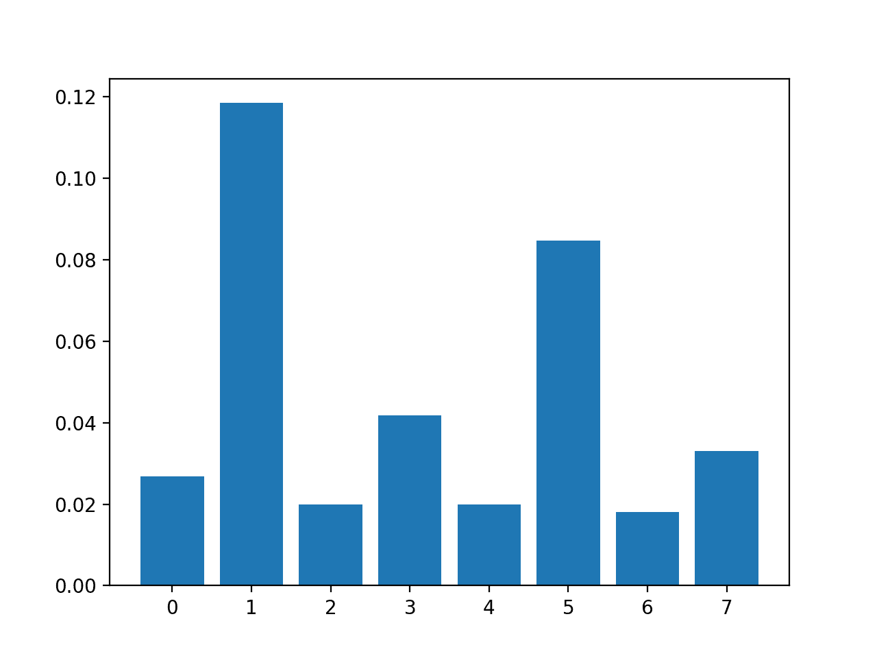
Bar Chart of the Input Features (x) vs. the Mutual Information Feature Importance (y)
Now that we know how to perform feature selection on numerical input data for a classification predictive modeling problem, we can try developing a model using the selected features and compare the results.
Modeling With Selected Features
There are many different techniques for scoring features and selecting features based on scores; how do you know which one to use?
A robust approach is to evaluate models using different feature selection methods (and numbers of features) and select the method that results in a model with the best performance.
In this section, we will evaluate a Logistic Regression model with all features compared to a model built from features selected by ANOVA f-test and those features selected via mutual information.
Logistic regression is a good model for testing feature selection methods as it can perform better if irrelevant features are removed from the model.
Model Built Using All Features
As a first step, we will evaluate a LogisticRegression model using all the available features.
The model is fit on the training dataset and evaluated on the test dataset.
The complete example is listed below.
|
1 2 3 4 5 6 7 8 9 10 11 12 13 14 15 16 17 18 19 20 21 22 23 24 25 26 27 28 29 |
# evaluation of a model using all input features from pandas import read_csv from sklearn.model_selection import train_test_split from sklearn.linear_model import LogisticRegression from sklearn.metrics import accuracy_score # load the dataset def load_dataset(filename): # load the dataset as a pandas DataFrame data = read_csv(filename, header=None) # retrieve numpy array dataset = data.values # split into input (X) and output (y) variables X = dataset[:, :-1] y = dataset[:,-1] return X, y # load the dataset X, y = load_dataset('pima-indians-diabetes.csv') # split into train and test sets X_train, X_test, y_train, y_test = train_test_split(X, y, test_size=0.33, random_state=1) # fit the model model = LogisticRegression(solver='liblinear') model.fit(X_train, y_train) # evaluate the model yhat = model.predict(X_test) # evaluate predictions accuracy = accuracy_score(y_test, yhat) print('Accuracy: %.2f' % (accuracy*100)) |
Running the example prints the accuracy of the model on the training dataset.
Note: Your results may vary given the stochastic nature of the algorithm or evaluation procedure, or differences in numerical precision. Consider running the example a few times and compare the average outcome.
In this case, we can see that the model achieves a classification accuracy of about 77 percent.
We would prefer to use a subset of features that achieves a classification accuracy that is as good or better than this.
|
1 |
Accuracy: 77.56 |
Model Built Using ANOVA f-test Features
We can use the ANOVA f-test to score the features and select the four most relevant features.
The select_features() function below is updated to achieve this.
|
1 2 3 4 5 6 7 8 9 10 11 |
# feature selection def select_features(X_train, y_train, X_test): # configure to select a subset of features fs = SelectKBest(score_func=f_classif, k=4) # learn relationship from training data fs.fit(X_train, y_train) # transform train input data X_train_fs = fs.transform(X_train) # transform test input data X_test_fs = fs.transform(X_test) return X_train_fs, X_test_fs, fs |
The complete example of evaluating a logistic regression model fit and evaluated on data using this feature selection method is listed below.
|
1 2 3 4 5 6 7 8 9 10 11 12 13 14 15 16 17 18 19 20 21 22 23 24 25 26 27 28 29 30 31 32 33 34 35 36 37 38 39 40 41 42 43 44 45 |
# evaluation of a model using 4 features chosen with anova f-test from pandas import read_csv from sklearn.model_selection import train_test_split from sklearn.feature_selection import SelectKBest from sklearn.feature_selection import f_classif from sklearn.linear_model import LogisticRegression from sklearn.metrics import accuracy_score # load the dataset def load_dataset(filename): # load the dataset as a pandas DataFrame data = read_csv(filename, header=None) # retrieve numpy array dataset = data.values # split into input (X) and output (y) variables X = dataset[:, :-1] y = dataset[:,-1] return X, y # feature selection def select_features(X_train, y_train, X_test): # configure to select a subset of features fs = SelectKBest(score_func=f_classif, k=4) # learn relationship from training data fs.fit(X_train, y_train) # transform train input data X_train_fs = fs.transform(X_train) # transform test input data X_test_fs = fs.transform(X_test) return X_train_fs, X_test_fs, fs # load the dataset X, y = load_dataset('pima-indians-diabetes.csv') # split into train and test sets X_train, X_test, y_train, y_test = train_test_split(X, y, test_size=0.33, random_state=1) # feature selection X_train_fs, X_test_fs, fs = select_features(X_train, y_train, X_test) # fit the model model = LogisticRegression(solver='liblinear') model.fit(X_train_fs, y_train) # evaluate the model yhat = model.predict(X_test_fs) # evaluate predictions accuracy = accuracy_score(y_test, yhat) print('Accuracy: %.2f' % (accuracy*100)) |
Running the example reports the performance of the model on just four of the eight input features selected using the ANOVA f-test statistic.
Note: Your results may vary given the stochastic nature of the algorithm or evaluation procedure, or differences in numerical precision. Consider running the example a few times and compare the average outcome.
In this case, we see that the model achieved an accuracy of about 78.74 percent, a lift in performance compared to the baseline that achieved 77.56 percent.
|
1 |
Accuracy: 78.74 |
Model Built Using Mutual Information Features
We can repeat the experiment and select the top four features using a mutual information statistic.
The updated version of the select_features() function to achieve this is listed below.
|
1 2 3 4 5 6 7 8 9 10 11 |
# feature selection def select_features(X_train, y_train, X_test): # configure to select a subset of features fs = SelectKBest(score_func=mutual_info_classif, k=4) # learn relationship from training data fs.fit(X_train, y_train) # transform train input data X_train_fs = fs.transform(X_train) # transform test input data X_test_fs = fs.transform(X_test) return X_train_fs, X_test_fs, fs |
The complete example of using mutual information for feature selection to fit a logistic regression model is listed below.
|
1 2 3 4 5 6 7 8 9 10 11 12 13 14 15 16 17 18 19 20 21 22 23 24 25 26 27 28 29 30 31 32 33 34 35 36 37 38 39 40 41 42 43 44 45 |
# evaluation of a model using 4 features chosen with mutual information from pandas import read_csv from sklearn.model_selection import train_test_split from sklearn.feature_selection import SelectKBest from sklearn.feature_selection import mutual_info_classif from sklearn.linear_model import LogisticRegression from sklearn.metrics import accuracy_score # load the dataset def load_dataset(filename): # load the dataset as a pandas DataFrame data = read_csv(filename, header=None) # retrieve numpy array dataset = data.values # split into input (X) and output (y) variables X = dataset[:, :-1] y = dataset[:,-1] return X, y # feature selection def select_features(X_train, y_train, X_test): # configure to select a subset of features fs = SelectKBest(score_func=mutual_info_classif, k=4) # learn relationship from training data fs.fit(X_train, y_train) # transform train input data X_train_fs = fs.transform(X_train) # transform test input data X_test_fs = fs.transform(X_test) return X_train_fs, X_test_fs, fs # load the dataset X, y = load_dataset('pima-indians-diabetes.csv') # split into train and test sets X_train, X_test, y_train, y_test = train_test_split(X, y, test_size=0.33, random_state=1) # feature selection X_train_fs, X_test_fs, fs = select_features(X_train, y_train, X_test) # fit the model model = LogisticRegression(solver='liblinear') model.fit(X_train_fs, y_train) # evaluate the model yhat = model.predict(X_test_fs) # evaluate predictions accuracy = accuracy_score(y_test, yhat) print('Accuracy: %.2f' % (accuracy*100)) |
Running the example fits the model on the four top selected features chosen using mutual information.
Note: Your results may vary given the stochastic nature of the algorithm or evaluation procedure, or differences in numerical precision. Consider running the example a few times and compare the average outcome.
In this case, we can make no difference compared to the baseline model. This is interesting as we know the method chose a different four features compared to the previous method.
|
1 |
Accuracy: 77.56 |
Tune the Number of Selected Features
In the previous example, we selected four features, but how do we know that is a good or best number of features to select?
Instead of guessing, we can systematically test a range of different numbers of selected features and discover which results in the best performing model. This is called a grid search, where the k argument to the SelectKBest class can be tuned.
It is good practice to evaluate model configurations on classification tasks using repeated stratified k-fold cross-validation. We will use three repeats of 10-fold cross-validation via the RepeatedStratifiedKFold class.
|
1 2 3 |
... # define the evaluation method cv = RepeatedStratifiedKFold(n_splits=10, n_repeats=3, random_state=1) |
We can define a Pipeline that correctly prepares the feature selection transform on the training set and applies it to the train set and test set for each fold of the cross-validation.
In this case, we will use the ANOVA f-test statistical method for selecting features.
|
1 2 3 4 5 |
... # define the pipeline to evaluate model = LogisticRegression(solver='liblinear') fs = SelectKBest(score_func=f_classif) pipeline = Pipeline(steps=[('anova',fs), ('lr', model)]) |
We can then define the grid of values to evaluate as 1 to 8.
Note that the grid is a dictionary of parameters to values to search, and given that we are using a Pipeline, we can access the SelectKBest object via the name we gave it, ‘anova‘, and then the parameter name ‘k‘, separated by two underscores, or ‘anova__k‘.
|
1 2 3 4 |
... # define the grid grid = dict() grid['anova__k'] = [i+1 for i in range(X.shape[1])] |
We can then define and run the search.
|
1 2 3 4 5 |
... # define the grid search search = GridSearchCV(pipeline, grid, scoring='accuracy', n_jobs=-1, cv=cv) # perform the search results = search.fit(X, y) |
Tying this together, the complete example is listed below.
|
1 2 3 4 5 6 7 8 9 10 11 12 13 14 15 16 17 18 19 20 21 22 23 24 25 26 27 28 29 30 31 32 33 34 35 36 37 38 39 |
# compare different numbers of features selected using anova f-test from pandas import read_csv from sklearn.model_selection import RepeatedStratifiedKFold from sklearn.feature_selection import SelectKBest from sklearn.feature_selection import f_classif from sklearn.linear_model import LogisticRegression from sklearn.pipeline import Pipeline from sklearn.model_selection import GridSearchCV from matplotlib import pyplot # load the dataset def load_dataset(filename): # load the dataset as a pandas DataFrame data = read_csv(filename, header=None) # retrieve numpy array dataset = data.values # split into input (X) and output (y) variables X = dataset[:, :-1] y = dataset[:,-1] return X, y # define dataset X, y = load_dataset('pima-indians-diabetes.csv') # define the evaluation method cv = RepeatedStratifiedKFold(n_splits=10, n_repeats=3, random_state=1) # define the pipeline to evaluate model = LogisticRegression(solver='liblinear') fs = SelectKBest(score_func=f_classif) pipeline = Pipeline(steps=[('anova',fs), ('lr', model)]) # define the grid grid = dict() grid['anova__k'] = [i+1 for i in range(X.shape[1])] # define the grid search search = GridSearchCV(pipeline, grid, scoring='accuracy', n_jobs=-1, cv=cv) # perform the search results = search.fit(X, y) # summarize best print('Best Mean Accuracy: %.3f' % results.best_score_) print('Best Config: %s' % results.best_params_) |
Running the example grid searches different numbers of selected features using ANOVA f-test, where each modeling pipeline is evaluated using repeated cross-validation.
Note: Your results may vary given the stochastic nature of the algorithm or evaluation procedure, or differences in numerical precision. Consider running the example a few times and compare the average outcome.
In this case, we can see that the best number of selected features is seven; that achieves an accuracy of about 77 percent.
|
1 2 |
Best Mean Accuracy: 0.770 Best Config: {'anova__k': 7} |
We might want to see the relationship between the number of selected features and classification accuracy. In this relationship, we may expect that more features result in a better performance to a point.
This relationship can be explored by manually evaluating each configuration of k for the SelectKBest from 1 to 8, gathering the sample of accuracy scores, and plotting the results using box and whisker plots side-by-side. The spread and mean of these box plots would be expected to show any interesting relationship between the number of selected features and the classification accuracy of the pipeline.
The complete example of achieving this is listed below.
|
1 2 3 4 5 6 7 8 9 10 11 12 13 14 15 16 17 18 19 20 21 22 23 24 25 26 27 28 29 30 31 32 33 34 35 36 37 38 39 40 41 42 43 44 45 46 47 48 |
# compare different numbers of features selected using anova f-test from numpy import mean from numpy import std from pandas import read_csv from sklearn.model_selection import cross_val_score from sklearn.model_selection import RepeatedStratifiedKFold from sklearn.feature_selection import SelectKBest from sklearn.feature_selection import f_classif from sklearn.linear_model import LogisticRegression from sklearn.pipeline import Pipeline from matplotlib import pyplot # load the dataset def load_dataset(filename): # load the dataset as a pandas DataFrame data = read_csv(filename, header=None) # retrieve numpy array dataset = data.values # split into input (X) and output (y) variables X = dataset[:, :-1] y = dataset[:,-1] return X, y # evaluate a give model using cross-validation def evaluate_model(model, X, y): cv = RepeatedStratifiedKFold(n_splits=10, n_repeats=3, random_state=1) scores = cross_val_score(model, X, y, scoring='accuracy', cv=cv, n_jobs=-1, error_score='raise') return scores # define dataset X, y = load_dataset('pima-indians-diabetes.csv') # define number of features to evaluate num_features = [i+1 for i in range(X.shape[1])] # enumerate each number of features results = list() for k in num_features: # create pipeline model = LogisticRegression(solver='liblinear') fs = SelectKBest(score_func=f_classif, k=k) pipeline = Pipeline(steps=[('anova',fs), ('lr', model)]) # evaluate the model scores = evaluate_model(pipeline, X, y) results.append(scores) # summarize the results print('>%d %.3f (%.3f)' % (k, mean(scores), std(scores))) # plot model performance for comparison pyplot.boxplot(results, labels=num_features, showmeans=True) pyplot.show() |
Running the example first reports the mean and standard deviation accuracy for each number of selected features.
Note: Your results may vary given the stochastic nature of the algorithm or evaluation procedure, or differences in numerical precision. Consider running the example a few times and compare the average outcome.
In this case, it looks like selecting five and seven features results in roughly the same accuracy.
|
1 2 3 4 5 6 7 8 |
>1 0.748 (0.048) >2 0.756 (0.042) >3 0.761 (0.044) >4 0.759 (0.042) >5 0.770 (0.041) >6 0.766 (0.042) >7 0.770 (0.042) >8 0.768 (0.040) |
Box and whisker plots are created side-by-side showing the trend of increasing mean accuracy with the number of selected features to five features, after which it may become less stable.
Selecting five features might be an appropriate configuration in this case.
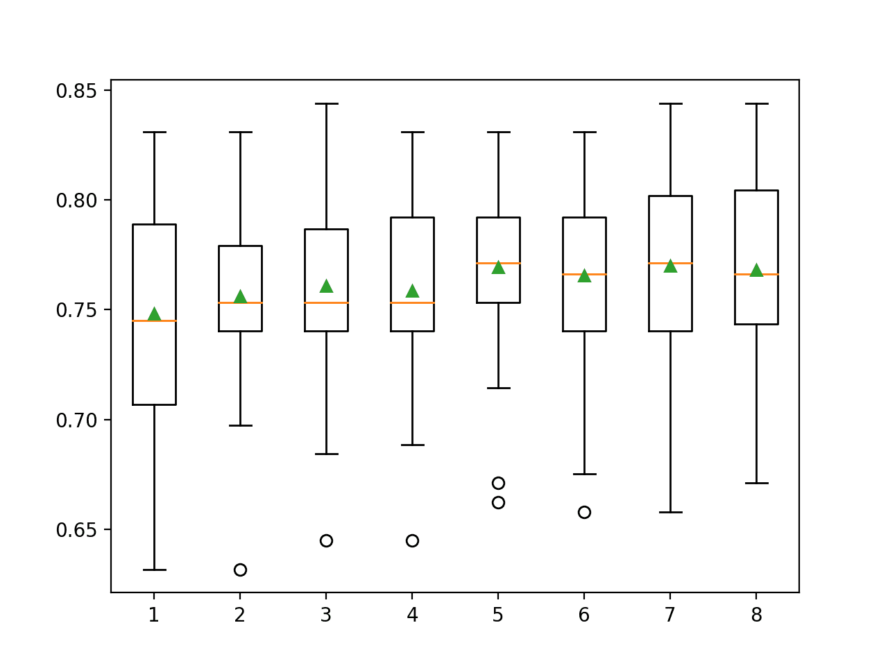
Box and Whisker Plots of Classification Accuracy for Each Number of Selected Features Using ANOVA f-test
Further Reading
This section provides more resources on the topic if you are looking to go deeper.
Tutorials
- How to Choose a Feature Selection Method For Machine Learning
- How to Perform Feature Selection with Categorical Data
- What Is Information Gain and Mutual Information for Machine Learning
Books
Papers
APIs
- Feature selection, Scikit-Learn User Guide.
- sklearn.feature_selection.f_classif API.
- sklearn.feature_selection.mutual_info_classif API.
- sklearn.feature_selection.SelectKBest API.
Articles
Datasets
- Diabetes Dataset (pima-indians-diabetes.csv)
- Diabetes Dataset Description (pima-indians-diabetes.names)
Summary
In this tutorial, you discovered how to perform feature selection with numerical input data for classification.
Specifically, you learned:
- The diabetes predictive modeling problem with numerical inputs and binary classification target variables.
- How to evaluate the importance of numerical features using the ANOVA f-test and mutual information statistics.
- How to perform feature selection for numerical data when fitting and evaluating a classification model.
Do you have any questions?
Ask your questions in the comments below and I will do my best to answer.


Great Motivation to us. Would you do for some stock prediction from NSE/BSE? How to apply feature selection for some equities and predict future price.
Thanks.
Probably not:
https://machinelearningmastery.com/faq/single-faq/can-you-help-me-with-machine-learning-for-finance-or-the-stock-market
This is excellent and so much helpful .. I am working on feature engineering and learning ..it’s vast what can be done
Thanks!
Jason, excellent post. Your code is always very concise and in the result one can cover it quickly eventhough it is highly technical. I read it because right now I am struggling with the same problem: figuring out the optimal number of features for a classifier, mainly to improve compute time. Question: you have done this for lLogisticRegression(solver=’liblinear’). We seem to have found the optimal number of features, but that’s for this particular estimator only, as I understand. Now however, can we generalize this lesson?
In other words, how can we infer this information on the optimal number of features to other classifiers, potentially working on the same set? I understand that the answer strongly depends on the type of classifier. I think there isn’t a short answer (or is there one?) and so perhaps you would like to consider a followup post in some time. In any case, the above is already very useful, thank you.
Thanks!
Great question.
No. You may need to test different representations with different models to flush out what works well/best for your dataset. If you see the same features/results across models, then you can say that the finding generalizes across models for your dataset.
Thanks a lot for your tutorials, they are always a great source of information and help.
Thanks!
Dear sir, Your post helpful and easy to understand each and every point u mentioned. thank you
Thanks, I’m happy to hear that.
Hi Jason,
Very helpful tutorial.
How do we know finally which features were selected after applying Grid SearchCV and RepeatedStratifiedKFold class.?
I mean what is the way to print them?
Thanks!!
We don’t.
Knowing what features give the best model performance solves a different problem from feature selection to learn more about the dataset.
E.g. in the latter case you can use the full dataset and the chosen configuration with a standalone modeling pipeline to list the selected features from the procedure.
Hi Jason,
Impressive tutorial! thanks.
To be honest I see many options (as much as yours many tutorials) to be tested in order to get the final features importance, reduction or selection of every particular problem. Do you have a full tutorial list on the subject?
Anyway, regarding “SelectKBest” I am pleasantly surprised by the example application I read on Sklearn function description:
https://scikit-learn.org/stable/modules/generated/sklearn.feature_selection.SelectKBest.html
That is that function can be applied also to Images dataset (not only tabular as it is this case)…e.g. I see in “load_digits” example that SelectKBest can calculate the Best 20 pixels of the 64 per image …so my questions are:
1) Is it true SelectKbest is also a valid method for computer vision?
2) In the example they choose to select finally 20 pixels from 64 = 8x 8 original…how I can know which pixels are finally the ones selected?
3) do you have any tutorial applying SelectKBest to imaging?
Thank you Jason
Thanks.
Not sure what you’re asking, you mean all data prep tutorials:
https://machinelearningmastery.com/category/data-preparation/
I’m surprised people are using feature selection on pixels, it seems mad to me off the cuff.
I have no examples of this, I need to think about it.
Hi Jason:
I experiment my self with the few simples codes lines, in the example presented on “SelectKBest()”:
regarding the above reflexion:
from sklearn.datasets import load_digits
from sklearn.feature_selection import SelectKBest, chi2
X, y = load_digits(return_X_y=True)
X.shape
(1797, 64)
X_new = SelectKBest(chi2, k=25).fit_transform(X, y)
X_new.shape
(1797, 25)
I decided to apply several Sklearn Models such as (Dummy(), logisticRegression(), SVC(), ExtraTreesClassifier(), RandomForestClassifier(), XGBClassifier(), GradientBoostingClassifier() and BaggingClassifier()), for Sklear digit dataset problem (I guess it is a simple version of 8 x 8 pixels imaging of MNIST currently 28 x 28).
And of course I compare vs the reduced images (instead of 64 pixels I decided to select the best 25 pixels -5×5-) and finally I compare the accuracy as metric evaluator and I get a little difference of less than 1 % on accuracy for reduced images of only 25 total pixels instead of 64.
So the conclusion is that we can reduce imaging pixels in order to get a simple and faster dataset training and we only lost 0.5% of accuracy ….so it is working !
I used dataset pixels normalization (between 0 and 1) but no labelling encoding at all with sklearn models…and for example I got 98.9 % accuracy with modelo SVC as the best model for image digits multi-classification …Even I plot the reduced images of only 5 x 5 pixels = 25 and I got the reduced features…that the machine can interpret pretty well but not myself (I could not recognised the figures or digits on it :-))
I am sure you will expand this new powerful tool of image reduction, using features reduction or selection techniques… on new tutorials, meanwhile I am happy to experiment with this techniques and open this door to everybody on your ML community…
so one more time your inspire us many to do many experiments with your awesome tutorials. Thank you Jason!
Very nice, thanks for sharing!
Hey Jason,
when selecting the number of features with ANOVA f-test statistic and my target variable is imbalanced…Is it right that I select the number of features first, then transform my input data (cause its not normally distributed) and upsample the minority class (e.g with smote) when the target variable is imbalanced? Or shall I do it in another order? Thanks in advance as always 😉
Yes, ideally you would apply data preparation like feature selection and changing probability distributions before using a knn-based resampling of rows.
Thank you Jason 🙂
You’re welcome.
Can we use these methods when the dataset contains numerical and categorical data? In my data set there are some numerical features and some categorical data which are replaced by Label Encoding features. What feature selection approaches are better to use?
The above are for numerical variables.
If you have both types of input data, you can use RFE:
https://machinelearningmastery.com/rfe-feature-selection-in-python/
Or a columntransformer:
https://machinelearningmastery.com/columntransformer-for-numerical-and-categorical-data/
Do we need to standardize before calculating mutual information for continuous variables?
Perhaps evaluate your model with and without scaling prior to selection and compare the results.
Thanks for this, i’ve read that selectkbest is normally only good for normally dsitributed features. I am using a tree-based model. I don’t therefore standardize/normalize but now i am wondering if using selectKbest was the best choice when my data does not hold the normal assumption.
Is this correct?
What non parametric feature selection methods can i use in sklearn?
Hi Zjo…The follow is an excellent resource for the usage of “selectkbest”.
https://www.datatechnotes.com/2021/02/seleckbest-feature-selection-example-in-python.html
The paper that you have referenced talks about nearest neighbor based modifications in the algorithm for such a task of numerical and continuous variable. The method described by you here is different.
Thank you for the feedback Anjali!
Thank you very much for your tutorial, I got a lot of information about feature selection.
I would like to ask a question related to feature selection
I have a dataset with 2 data types, categorical and numeric. The target is categorical with (0 and 1). I did ANOVA for numeric data type and chi-square for categorical data. However, when I tested my numeric data, no features were selected. So, when I looked at the suggestions in the comments, I saw a suggestion to use RFE. But I was overwhelmed to make it because I used modeling using ANN – Backpropagation algorithm. To handle this problem, do you have a source or tutorial as a reference material?
Thank you.
Hi Dede…You are very welcome! The following resource may be helpful to decide a feature selection method:
https://machinelearningmastery.com/feature-selection-with-real-and-categorical-data/
Hi Jason,
Thanks for the great article.
I have a question regarding prerequisites for anova ftest.
“In order to use an ANOVA F-Test, each group must be normally distributed”.
How we can ensure that the data is normally distributed?
Which step in this example makes the data normally distributed.
If the dataset does not have normal distribution, can we use anova?
Are we using one way anova or two way anova here. I am sorry if i am asking basics….