Datasets may have missing values, and this can cause problems for many machine learning algorithms.
As such, it is good practice to identify and replace missing values for each column in your input data prior to modeling your prediction task. This is called missing data imputation, or imputing for short.
A popular approach to missing data imputation is to use a model to predict the missing values. This requires a model to be created for each input variable that has missing values. Although any one among a range of different models can be used to predict the missing values, the k-nearest neighbor (KNN) algorithm has proven to be generally effective, often referred to as “nearest neighbor imputation.”
In this tutorial, you will discover how to use nearest neighbor imputation strategies for missing data in machine learning.
After completing this tutorial, you will know:
Missing values must be marked with NaN values and can be replaced with nearest neighbor estimated values.
How to load a CSV file with missing values and mark the missing values with NaN values and report the number and percentage of missing values for each column.
How to impute missing values with nearest neighbor models as a data preparation method when evaluating models and when fitting a final model to make predictions on new data.
Kick-start your project with my new book Data Preparation for Machine Learning, including step-by-step tutorials and the Python source code files for all examples.
Let’s get started.
Updated Jun/2020: Changed the column used for prediction in examples.
kNN Imputation for Missing Values in Machine Learning Photo by portengaround, some rights reserved.
Tutorial Overview
This tutorial is divided into three parts; they are:
k-Nearest Neighbor Imputation
Horse Colic Dataset
Nearest Neighbor Imputation With KNNImputer
KNNImputer Data Transform
KNNImputer and Model Evaluation
KNNImputer and Different Number of Neighbors
KNNImputer Transform When Making a Prediction
k-Nearest Neighbor Imputation
A dataset may have missing values.
These are rows of data where one or more values or columns in that row are not present. The values may be missing completely or they may be marked with a special character or value, such as a question mark “?“.
Values could be missing for many reasons, often specific to the problem domain, and might include reasons such as corrupt measurements or unavailability.
Most machine learning algorithms require numeric input values, and a value to be present for each row and column in a dataset. As such, missing values can cause problems for machine learning algorithms.
It is common to identify missing values in a dataset and replace them with a numeric value. This is called data imputing, or missing data imputation.
… missing data can be imputed. In this case, we can use information in the training set predictors to, in essence, estimate the values of other predictors.
An effective approach to data imputing is to use a model to predict the missing values. A model is created for each feature that has missing values, taking as input values of perhaps all other input features.
One popular technique for imputation is a K-nearest neighbor model. A new sample is imputed by finding the samples in the training set “closest” to it and averages these nearby points to fill in the value.
If input variables are numeric, then regression models can be used for prediction, and this case is quite common. A range of different models can be used, although a simple k-nearest neighbor (KNN) model has proven to be effective in experiments. The use of a KNN model to predict or fill missing values is referred to as “Nearest Neighbor Imputation” or “KNN imputation.”
We show that KNNimpute appears to provide a more robust and sensitive method for missing value estimation […] and KNNimpute surpass the commonly used row average method (as well as filling missing values with zeros).
Configuration of KNN imputation often involves selecting the distance measure (e.g. Euclidean) and the number of contributing neighbors for each prediction, the k hyperparameter of the KNN algorithm.
Now that we are familiar with nearest neighbor methods for missing value imputation, let’s take a look at a dataset with missing values.
Want to Get Started With Data Preparation?
Take my free 7-day email crash course now (with sample code).
Click to sign-up and also get a free PDF Ebook version of the course.
Horse Colic Dataset
The horse colic dataset describes medical characteristics of horses with colic and whether they lived or died.
There are 300 rows and 26 input variables with one output variable. It is a binary classification prediction task that involves predicting 1 if the horse lived and 2 if the horse died.
There are many fields we could select to predict in this dataset. In this case, we will predict whether the problem was surgical or not (column index 23), making it a binary classification problem.
The dataset has many missing values for many of the columns where each missing value is marked with a question mark character (“?”).
Below provides an example of rows from the dataset with marked missing values.
4 2.0 1 530255 37.3 104.0 35.0 NaN ... NaN 2.0 2 4300 0 0 2
[5 rows x 28 columns]
Next, we can see a list of all columns in the dataset and the number and percentage of missing values.
We can see that some columns (e.g. column indexes 1 and 2) have no missing values and other columns (e.g. column indexes 15 and 21) have many or even a majority of missing values.
1
2
3
4
5
6
7
8
9
10
11
12
13
14
15
16
17
18
19
20
21
22
23
24
25
26
27
28
> 0, Missing: 1 (0.3%)
> 1, Missing: 0 (0.0%)
> 2, Missing: 0 (0.0%)
> 3, Missing: 60 (20.0%)
> 4, Missing: 24 (8.0%)
> 5, Missing: 58 (19.3%)
> 6, Missing: 56 (18.7%)
> 7, Missing: 69 (23.0%)
> 8, Missing: 47 (15.7%)
> 9, Missing: 32 (10.7%)
> 10, Missing: 55 (18.3%)
> 11, Missing: 44 (14.7%)
> 12, Missing: 56 (18.7%)
> 13, Missing: 104 (34.7%)
> 14, Missing: 106 (35.3%)
> 15, Missing: 247 (82.3%)
> 16, Missing: 102 (34.0%)
> 17, Missing: 118 (39.3%)
> 18, Missing: 29 (9.7%)
> 19, Missing: 33 (11.0%)
> 20, Missing: 165 (55.0%)
> 21, Missing: 198 (66.0%)
> 22, Missing: 1 (0.3%)
> 23, Missing: 0 (0.0%)
> 24, Missing: 0 (0.0%)
> 25, Missing: 0 (0.0%)
> 26, Missing: 0 (0.0%)
> 27, Missing: 0 (0.0%)
Now that we are familiar with the horse colic dataset that has missing values, let’s look at how we can use nearest neighbor imputation.
Nearest Neighbor Imputation with KNNImputer
The scikit-learn machine learning library provides the KNNImputer class that supports nearest neighbor imputation.
In this section, we will explore how to effectively use the KNNImputer class.
KNNImputer Data Transform
KNNImputer is a data transform that is first configured based on the method used to estimate the missing values.
The default distance measure is a Euclidean distance measure that is NaN aware, e.g. will not include NaN values when calculating the distance between members of the training dataset. This is set via the “metric” argument.
The number of neighbors is set to five by default and can be configured by the “n_neighbors” argument.
Finally, the distance measure can be weighed proportional to the distance between instances (rows), although this is set to a uniform weighting by default, controlled via the “weights” argument.
Then, the fit imputer is applied to a dataset to create a copy of the dataset with all missing values for each column replaced with an estimated value.
1
2
3
...
# transform the dataset
Xtrans=imputer.transform(X)
We can demonstrate its usage on the horse colic dataset and confirm it works by summarizing the total number of missing values in the dataset before and after the transform.
The complete example is listed below.
1
2
3
4
5
6
7
8
9
10
11
12
13
14
15
16
17
18
19
20
21
# knn imputation transform for the horse colic dataset
Running the example first loads the dataset and reports the total number of missing values in the dataset as 1,605.
The transform is configured, fit, and performed, and the resulting new dataset has no missing values, confirming it was performed as we expected.
Each missing value was replaced with a value estimated by the model.
1
2
Missing: 1605
Missing: 0
KNNImputer and Model Evaluation
It is a good practice to evaluate machine learning models on a dataset using k-fold cross-validation.
To correctly apply nearest neighbor missing data imputation and avoid data leakage, it is required that the models are calculated for each column are calculated on the training dataset only, then applied to the train and test sets for each fold in the dataset.
This can be achieved by creating a modeling pipeline where the first step is the nearest neighbor imputation, then the second step is the model. This can be achieved using the Pipeline class.
For example, the Pipeline below uses a KNNImputer with the default strategy, followed by a random forest model.
Running the example correctly applies data imputation to each fold of the cross-validation procedure.
Note: Your results may vary given the stochastic nature of the algorithm or evaluation procedure, or differences in numerical precision. Consider running the example a few times and compare the average outcome.
The pipeline is evaluated using three repeats of 10-fold cross-validation and reports the mean classification accuracy on the dataset as about 86.2 percent, which is a reasonable score.
1
Mean Accuracy: 0.862 (0.059)
How do we know that using a default number of neighbors of five is good or best for this dataset?
The answer is that we don’t.
KNNImputer and Different Number of Neighbors
The key hyperparameter for the KNN algorithm is k; that controls the number of nearest neighbors that are used to contribute to a prediction.
It is good practice to test a suite of different values for k.
The example below evaluates model pipelines and compares odd values for k from 1 to 21.
1
2
3
4
5
6
7
8
9
10
11
12
13
14
15
16
17
18
19
20
21
22
23
24
25
26
27
28
29
30
31
32
# compare knn imputation strategies for the horse colic dataset
from numpy import mean
from numpy import std
from pandas import read_csv
from sklearn.ensemble import RandomForestClassifier
from sklearn.impute import KNNImputer
from sklearn.model_selection import cross_val_score
from sklearn.model_selection import RepeatedStratifiedKFold
Running the example evaluates each k value on the horse colic dataset using repeated cross-validation.
Note: Your results may vary given the stochastic nature of the algorithm or evaluation procedure, or differences in numerical precision. Consider running the example a few times and compare the average outcome.
The mean classification accuracy is reported for the pipeline with each k value used for imputation.
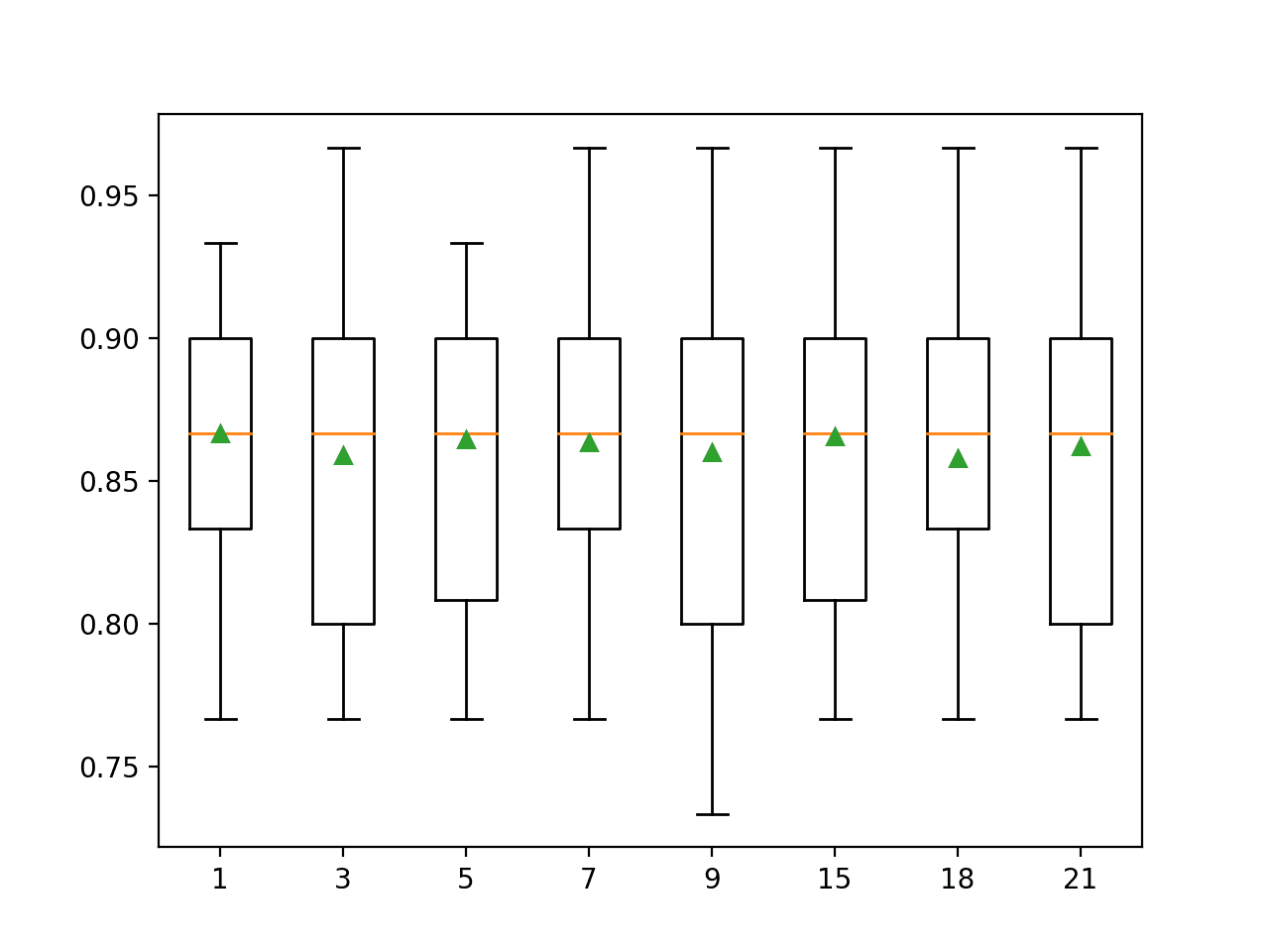
In this case, we can see that larger k values result in a better performing model, with a k=1 resulting in the best performance of about 86.7 percent accuracy.
1
2
3
4
5
6
7
8
>1 0.867 (0.049)
>3 0.859 (0.056)
>5 0.864 (0.054)
>7 0.863 (0.053)
>9 0.860 (0.062)
>15 0.866 (0.054)
>18 0.858 (0.052)
>21 0.862 (0.056)
At the end of the run, a box and whisker plot is created for each set of results, allowing the distribution of results to be compared.
The plot suggest that there is not much difference in the k value when imputing the missing values, with minor fluctuations around the mean performance (green triangle).
Box and Whisker Plot of Imputation Number of Neighbors for the Horse Colic Dataset
KNNImputer Transform When Making a Prediction
We may wish to create a final modeling pipeline with the nearest neighbor imputation and random forest algorithm, then make a prediction for new data.
This can be achieved by defining the pipeline and fitting it on all available data, then calling the predict() function, passing new data in as an argument.
Importantly, the row of new data must mark any missing values using the NaN value.
In this tutorial, you discovered how to use nearest neighbor imputation strategies for missing data in machine learning.
Specifically, you learned:
Missing values must be marked with NaN values and can be replaced with nearest neighbor estimated values.
How to load a CSV file with missing values and mark the missing values with NaN values and report the number and percentage of missing values for each column.
How to impute missing values with nearest neighbor models as a data preparation method when evaluating models and when fitting a final model to make predictions on new data.
Do you have any questions?
Ask your questions in the comments below and I will do my best to answer.
It provides self-study tutorials with full working code on: Feature Selection, RFE, Data Cleaning, Data Transforms, Scaling, Dimensionality Reduction,
and much more...
Bring Modern Data Preparation Techniques to Your Machine Learning Projects
When I explicitly trained the model on the imputed data (without cross-validation), I got an accuracy of 1.0 for the training dataset. A very big concern!. what do you think might be wrong?. Check the code below for clarity.
import numpy as np
from pandas import read_csv
from sklearn.ensemble import RandomForestClassifier
from sklearn.impute import KNNImputer
from sklearn.pipeline import Pipeline
Great post Jason!
I think that a wrong column was taken as a “y”/prediction. Last column refers to “cp_data” (if a pathology is present or not, and according to “horse-colic.names” is of no significance since pathology data is not included or collected for these cases).
I guess the prediction should be done over 23th-column; “outcome” with values 1 = lived,2 = died or 3 = was euthanized.
How we can evaluate only the Knn-imputer? I mean if for example, we want to compare the performance of two different imputers in a dataset how we can test them?
Hi Jason this is a great tutorial, thank you!
I have a problem when using KNN imputer on a relatively larger dataset.
I tried it out on a dataset –about 100K rows and 50 features. When I impute missing values using this method, I hit memory problems. Should I fit and transform by chunk (i.e iterate on every 1000 rows or so?) I am not sure if this is a good way to solve this issue.
Perhaps you can try on a machine with more memory?
Perhaps you can use a smaller sample of your dataset to fit the imputer then apply it?
Perhaps you can use a different imputer technique, like the statistical method?
Hi Jason, thanks for the tutorial! I applied this code to my train dataset however, the test set also includes missing values. So, should I create a KNN imputer for the test set also?
Hello Jason, thanks for this blog.
I have a dataset with the shape of 56K X 52, after applying the KNN imputation to my dataset I noticed the columns increased from 52 to 97, what could go be wrong?
I’m clueless , thanks.
Hello jason , thanks for blog .
Why dont you create a code for handling missing value treatment with different types like mean ,median and data scaling techniques all together . Actually that helps me a lot.
Thanking in advance
Thank you for the article – it’s very impressive. Is there a repo I can use as a reference? I checked GitHub and looks like you don’t have anything public.
I wondered whether there was any need to scale the data before imputation (as I have seen this mentioned elsewhere)?
I am using this imputer at the start of my pipeline for a random forest regressor. The dataset, like the one in your example contains un-scaled features.
Hi Jason, many thanks for this, quick question, if you have created a pipeline, imputed missing values with KNN how would you then save this (eg pickle) so that when you supply a small live daily data file to the model it carries out all the operations in particular the KNN impute. Does it store the whole of the training file and hence enabling it to calculate missing values on the fresh data. I can see perhaps that with regression impute it creates a regression formula which can be stored but what about KNN
Do you have any material coming up on imputing missing values on time series utilising other variables too? I’ve seen some papers using NN such as the following but no implementations.
Hi Jason,
Trying to implement a KNN imputation for a recommender system problem.
Is there a way to change the distance from euclidean to cosine distance?
Thanks,
Ritvik
In my case, after running ‘KNNimputer’, number of columns was reduced which is I guess because multiple columns that have no value at all were removed. The resulting columns were named as ‘1,2,3,…’. How can I retrieve column names?
Thank you for the post; it is very interesting and provides a thorough explanation of the KNN imputation technique 🙂
I wanted to ask about more details regarding the comparison of KNN and other imputation techniques (e.g., MICE). Specifically, when would it be better (and why would we prefer) to use KNN relative to MICE?
Hey james, I was wandering if it is a good approach normalize the variables befoe applying the KNN imputetion since it is based on euclidian distance?!
Hi Mehrdad….For studying the theory of machine learning-based imputation methods such as k-nearest neighbors (KNN) imputation and support vector machines (SVM) imputation, the following book is highly recommended:
### Book Recommendation
**”Data Mining: Concepts and Techniques” by Jiawei Han, Micheline Kamber, and Jian Pei**
This book provides a comprehensive introduction to data mining and includes detailed discussions on various imputation methods. While it covers a broad range of topics in data mining, it includes sections on missing data handling and imputation techniques.
### Additional Resources
1. **”Pattern Recognition and Machine Learning” by Christopher M. Bishop**
– This book provides a solid foundation in machine learning and includes discussions on various algorithms, including KNN and SVM. It also touches on data preprocessing techniques, which include imputation methods.
2. **Research Papers and Articles**
– For more specific and advanced techniques, you can look into research papers available on platforms like Google Scholar or arXiv. Search for terms like “KNN imputation methods,” “SVM imputation methods,” and “machine learning imputation.”
3. **Online Tutorials and Courses**
– Websites like Coursera, edX, and Udacity offer courses on machine learning that include modules on data preprocessing and imputation methods. These can provide practical insights along with theoretical knowledge.
### Online Resources
– **Google Scholar**: Search for “KNN imputation” and “SVM imputation” for academic papers.
– **arXiv**: Use the same search terms to find preprints of research papers.
These resources should give you a comprehensive understanding of the theory and application of machine learning-based imputation methods.


Can we apply knn imputation for cases where missing value percentage is greater than 95%, also should we process such features?
Ouch.
Perhaps, but the imputed values might not add a lot of value. Test and see.
excellent blog…..
but we have to see what would be the value
You must try it and discover if it offers value for your project.
When I explicitly trained the model on the imputed data (without cross-validation), I got an accuracy of 1.0 for the training dataset. A very big concern!. what do you think might be wrong?. Check the code below for clarity.
import numpy as np
from pandas import read_csv
from sklearn.ensemble import RandomForestClassifier
from sklearn.impute import KNNImputer
from sklearn.pipeline import Pipeline
# load dataset
url = ‘https://raw.githubusercontent.com/jbrownlee/Datasets/master/horse-colic.csv’
data = read_csv(url, header=None, na_values=’?’)
ix = [i for i in range(data.shape[1]) if i !=23]
y, X = data.values[:, 23], data.values[:,ix]
model = RandomForestClassifier()
imputer = KNNImputer()
pipeline = Pipeline(steps=[(‘i’, imputer), (‘m’, model)])
pipeline.fit(X,y)
print(pipeline.score(X,y))
#output
1.0
[program finished]
Accuracy should always be 100% on train in the best case.
Ignore performance on train, focus on performance on the hold out set.
Great post Jason!
I think that a wrong column was taken as a “y”/prediction. Last column refers to “cp_data” (if a pathology is present or not, and according to “horse-colic.names” is of no significance since pathology data is not included or collected for these cases).
I guess the prediction should be done over 23th-column; “outcome” with values 1 = lived,2 = died or 3 = was euthanized.
I think you’re right, I’l update it.
Hey Jason I was wondering whether it is possible to apply knn imputation for time series too?
Perhaps. I would guess that persistence would be a better approach.
Hi, Thank you for the great tutorial.
How we can evaluate only the Knn-imputer? I mean if for example, we want to compare the performance of two different imputers in a dataset how we can test them?
Thanks
Evaluate the model trained on the imputed data.
Hi Jason this is a great tutorial, thank you!
I have a problem when using KNN imputer on a relatively larger dataset.
I tried it out on a dataset –about 100K rows and 50 features. When I impute missing values using this method, I hit memory problems. Should I fit and transform by chunk (i.e iterate on every 1000 rows or so?) I am not sure if this is a good way to solve this issue.
Thanks!
Sorry to hear that.
Perhaps you can try on a machine with more memory?
Perhaps you can use a smaller sample of your dataset to fit the imputer then apply it?
Perhaps you can use a different imputer technique, like the statistical method?
Hi Jason, thanks for the tutorial! I applied this code to my train dataset however, the test set also includes missing values. So, should I create a KNN imputer for the test set also?
Fit the transform on the training set then apply it on the training set and the test set.
Or use a pipeline to handle this automatically.
Hello Jason, thanks for this blog.
I have a dataset with the shape of 56K X 52, after applying the KNN imputation to my dataset I noticed the columns increased from 52 to 97, what could go be wrong?
I’m clueless , thanks.
I don’t know, perhaps try debugging your code to find the cause.
Hello jason , thanks for blog .
Why dont you create a code for handling missing value treatment with different types like mean ,median and data scaling techniques all together . Actually that helps me a lot.
Thanking in advance
I have, you can find it here:
https://machinelearningmastery.com/statistical-imputation-for-missing-values-in-machine-learning/
Hi Jason,
Thank you for the article – it’s very impressive. Is there a repo I can use as a reference? I checked GitHub and looks like you don’t have anything public.
Thanks.
Yes, I don’t provide code via github repos, this is intentional. I prefer to provide the full context for the code with tutorials.
You can copy the code directly from the tutorial:
https://machinelearningmastery.com/faq/single-faq/how-do-i-copy-code-from-a-tutorial
Code files are provided with the tutorial books:
https://machinelearningmastery.com/products/
from sklearn.impute import KNNImputer
ImportError: cannot import name ‘KNNImputer’ from ‘sklearn.impute’ (C:\ProgramData\Anaconda3\lib\site-packages\sklearn\impute.py)
python 3.7 fails
how to fix
You need to update your version of the scikit-learn library.
Hi Jason,
Thank you for a great article/tutorial.
I wondered whether there was any need to scale the data before imputation (as I have seen this mentioned elsewhere)?
I am using this imputer at the start of my pipeline for a random forest regressor. The dataset, like the one in your example contains un-scaled features.
You’re welcome.
Yes, scaling before imputation can help if you have variables with different scales.
How do we apply KNNImpute for Categorical features?
Perhaps ordinal encode the values then apply as per normal.
Hi Jason,
Thanks for the reply.
Is it the right approach to apply ordinal encoding to the nominal categorical features?
and what are the other ways of handling missing values in categorical features?
Yes, you can use ordinal encoding, replace missing with the “statistical mode”, then one hot encode or whatever you like to start modeling.
Hi Jason, many thanks for this, quick question, if you have created a pipeline, imputed missing values with KNN how would you then save this (eg pickle) so that when you supply a small live daily data file to the model it carries out all the operations in particular the KNN impute. Does it store the whole of the training file and hence enabling it to calculate missing values on the fresh data. I can see perhaps that with regression impute it creates a regression formula which can be stored but what about KNN
You’re welcome.
You can pickle the pipeline directly.
Yes, if a knn impute is used, it will save whatever it needs to impute in the future – e.g. a kd-tree of the training data.
Hello and thanks for this great tutorial. I was wondering if there is there a reference available for this part: KNNImputer and Model Evaluation.
See the “further reading” section.
HI Jason, loving your site!
Do you have any material coming up on imputing missing values on time series utilising other variables too? I’ve seen some papers using NN such as the following but no implementations.
https://uwspace.uwaterloo.ca/bitstream/handle/10012/16561/Saad_Muhammad.pdf?sequence=5&isAllowed=y
https://ieeexplore.ieee.org/abstract/document/8904638
Thanks!
Thanks!
Yes:
https://machinelearningmastery.com/handle-missing-timesteps-sequence-prediction-problems-python/
Can we apply KNN imputation row-wise?
Perhaps. You may have to write custom code.
Hi Jason,
Trying to implement a KNN imputation for a recommender system problem.
Is there a way to change the distance from euclidean to cosine distance?
Thanks,
Ritvik
Yes, I believe you can specify the knn model with any distance metric you want.
Hi Jason,
Which is the best way to impute nans in categorical variables? I use ‘zzz’ or mode, but i’m not happy with that.
thanks man
There are many ways to perform imputation, try a suite of methods and discover what works best for your model and dataset.
In my case, after running ‘KNNimputer’, number of columns was reduced which is I guess because multiple columns that have no value at all were removed. The resulting columns were named as ‘1,2,3,…’. How can I retrieve column names?
Hi Cho…the following discussion is a great resource that will hopefully add clarity:
https://datascience.stackexchange.com/questions/65968/retrieve-dropped-column-names-from-sklearn-impute-simpleimputer
Hi Jason!
Thank you for the post; it is very interesting and provides a thorough explanation of the KNN imputation technique 🙂
I wanted to ask about more details regarding the comparison of KNN and other imputation techniques (e.g., MICE). Specifically, when would it be better (and why would we prefer) to use KNN relative to MICE?
Thanks in advance!
Endrit
Hi Endrit…The following may be of interest to you:
https://www.numpyninja.com/post/mice-and-knn-missing-value-imputations-through-python
Hey, I wanted to know how you extract the imputed dataframe from this pipeline? Thanks
Hi Dora…The following resources should add clarity:
https://medium.com/@kyawsawhtoon/a-guide-to-knn-imputation-95e2dc496e
https://www.analyticsvidhya.com/blog/2020/07/knnimputer-a-robust-way-to-impute-missing-values-using-scikit-learn/
Hey james, I was wandering if it is a good approach normalize the variables befoe applying the KNN imputetion since it is based on euclidian distance?!
Hi Caio…It is a good approach! More information can be found here:
https://medium.com/@kyawsawhtoon/a-guide-to-knn-imputation-95e2dc496e#:~:text=Another%20critical%20point%20here%20is,replacements%20for%20the%20missing%20values.
hello i need one book or file for study abut theory of machine learning base imputation method such as knn imputation svm imputation ,…
Hi Mehrdad….For studying the theory of machine learning-based imputation methods such as k-nearest neighbors (KNN) imputation and support vector machines (SVM) imputation, the following book is highly recommended:
### Book Recommendation
**”Data Mining: Concepts and Techniques” by Jiawei Han, Micheline Kamber, and Jian Pei**
This book provides a comprehensive introduction to data mining and includes detailed discussions on various imputation methods. While it covers a broad range of topics in data mining, it includes sections on missing data handling and imputation techniques.
### Additional Resources
1. **”Pattern Recognition and Machine Learning” by Christopher M. Bishop**
– This book provides a solid foundation in machine learning and includes discussions on various algorithms, including KNN and SVM. It also touches on data preprocessing techniques, which include imputation methods.
2. **Research Papers and Articles**
– For more specific and advanced techniques, you can look into research papers available on platforms like Google Scholar or arXiv. Search for terms like “KNN imputation methods,” “SVM imputation methods,” and “machine learning imputation.”
3. **Online Tutorials and Courses**
– Websites like Coursera, edX, and Udacity offer courses on machine learning that include modules on data preprocessing and imputation methods. These can provide practical insights along with theoretical knowledge.
### Online Resources
– **Google Scholar**: Search for “KNN imputation” and “SVM imputation” for academic papers.
– **arXiv**: Use the same search terms to find preprints of research papers.
These resources should give you a comprehensive understanding of the theory and application of machine learning-based imputation methods.