It can be challenging to develop a neural network predictive model for a new dataset.
One approach is to first inspect the dataset and develop ideas for what models might work, then explore the learning dynamics of simple models on the dataset, then finally develop and tune a model for the dataset with a robust test harness.
This process can be used to develop effective neural network models for classification and regression predictive modeling problems.
In this tutorial, you will discover how to develop a Multilayer Perceptron neural network model for the cancer survival binary classification dataset.
After completing this tutorial, you will know:
How to load and summarize the cancer survival dataset and use the results to suggest data preparations and model configurations to use.
How to explore the learning dynamics of simple MLP models on the dataset.
How to develop robust estimates of model performance, tune model performance and make predictions on new data.
Let’s get started.
Develop a Neural Network for Cancer Survival Dataset Photo by Bernd Thaller, some rights reserved.
Tutorial Overview
This tutorial is divided into 4 parts; they are:
Haberman Breast Cancer Survival Dataset
Neural Network Learning Dynamics
Robust Model Evaluation
Final Model and Make Predictions
Haberman Breast Cancer Survival Dataset
The first step is to define and explore the dataset.
We will be working with the “haberman” standard binary classification dataset.
The dataset describes breast cancer patient data and the outcome is patient survival. Specifically whether the patient survived for five years or longer, or whether the patient did not survive.
This is a standard dataset used in the study of imbalanced classification. According to the dataset description, the operations were conducted between 1958 and 1970 at the University of Chicago’s Billings Hospital.
There are 306 examples in the dataset, and there are 3 input variables; they are:
The age of the patient at the time of the operation.
The two-digit year of the operation.
The number of “positive axillary nodes” detected, a measure of whether cancer has spread.
As such, we have no control over the selection of cases that make up the dataset or features to use in those cases, other than what is available in the dataset.
Although the dataset describes breast cancer patient survival, given the small dataset size and the fact the data is based on breast cancer diagnosis and operations many decades ago, any models built on this dataset are not expected to generalize.
Note: to be crystal clear, we are NOT “solving breast cancer“. We are exploring a standard classification dataset.
Below is a sample of the first 5 rows of the dataset
Running the example loads the dataset directly from the URL and reports the shape of the dataset.
In this case, we can confirm that the dataset has 4 variables (3 input and one output) and that the dataset has 306 rows of data.
This is not many rows of data for a neural network and suggests that a small network, perhaps with regularization, would be appropriate.
It also suggests that using k-fold cross-validation would be a good idea given that it will give a more reliable estimate of model performance than a train/test split and because a single model will fit in seconds instead of hours or days with the largest datasets.
1
(306, 4)
Next, we can learn more about the dataset by looking at summary statistics and a plot of the data.
1
2
3
4
5
6
7
8
9
10
11
12
# show summary statistics and plots of the haberman dataset
Running the example first loads the data before and then prints summary statistics for each variable.
We can see that values vary with different means and standard deviations, perhaps some normalization or standardization would be required prior to modeling.
1
2
3
4
5
6
7
8
9
0 1 2 3
count 306.000000 306.000000 306.000000 306.000000
mean 52.457516 62.852941 4.026144 1.264706
std 10.803452 3.249405 7.189654 0.441899
min 30.000000 58.000000 0.000000 1.000000
25% 44.000000 60.000000 0.000000 1.000000
50% 52.000000 63.000000 1.000000 1.000000
75% 60.750000 65.750000 4.000000 2.000000
max 83.000000 69.000000 52.000000 2.000000
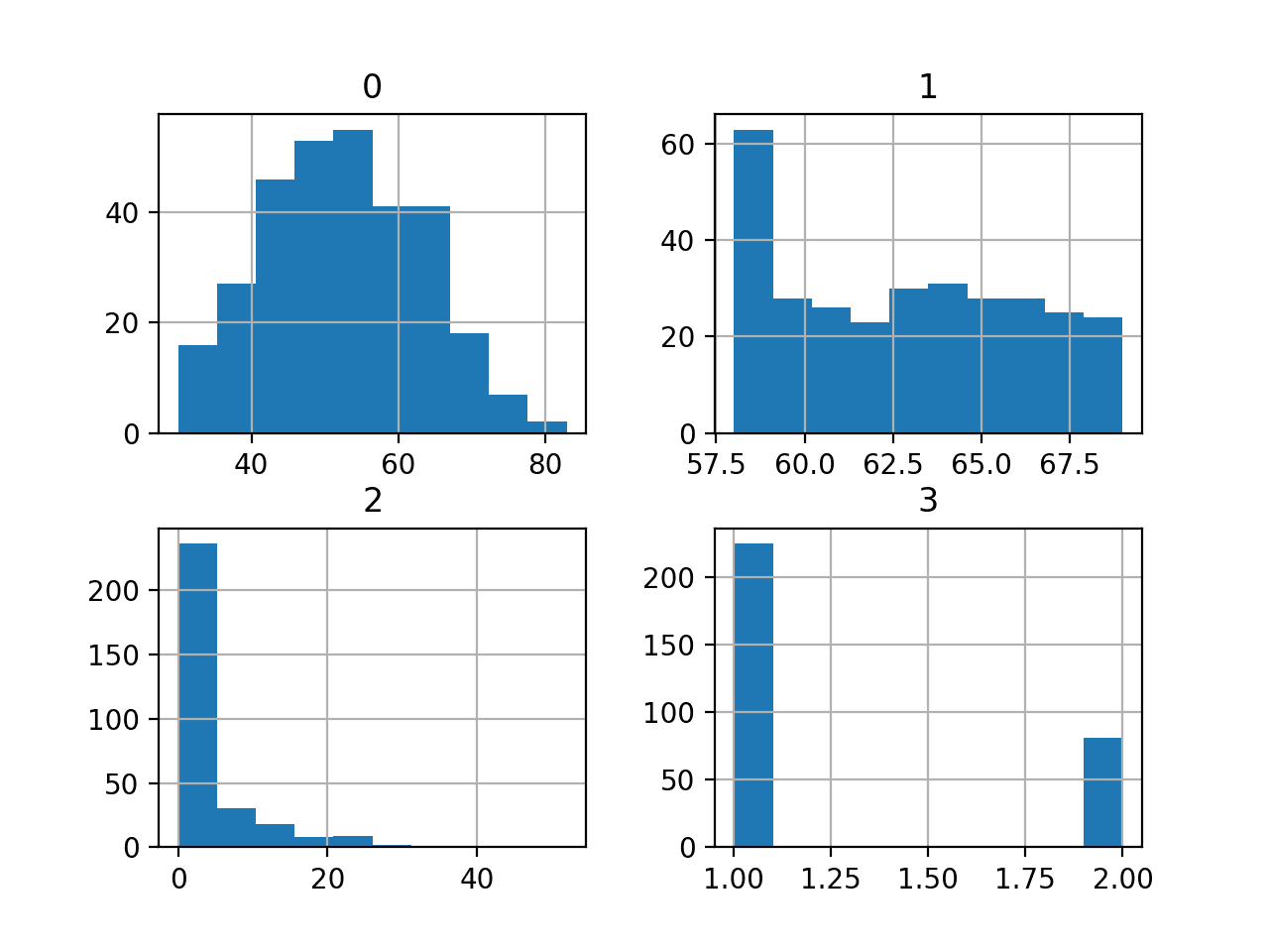
A histogram plot is then created for each variable.
We can see that perhaps the first variable has a Gaussian-like distribution and the next two input variables may have an exponential distribution.
We may have some benefit in using a power transform on each variable in order to make the probability distribution less skewed which will likely improve model performance.
Histograms of the Haberman Breast Cancer Survival Classification Dataset
We can see some skew in the distribution of examples between the two classes, meaning that the classification problem is not balanced. It is imbalanced.
It may be helpful to know how imbalanced the dataset actually is.
We can use the Counter object to count the number of examples in each class, then use those counts to summarize the distribution.
The complete example is listed below.
1
2
3
4
5
6
7
8
9
10
11
12
13
14
15
# summarize the class ratio of the haberman dataset
Running the example summarizes the class distribution for the dataset.
We can see that class 1 for survival has the most examples at 225, or about 74 percent of the dataset. We can see class 2 for non-survival has fewer examples at 81, or about 26 percent of the dataset.
The class distribution is skewed, but it is not severely imbalanced.
1
2
Class=1, Count=225, Percentage=73.529%
Class=2, Count=81, Percentage=26.471%
This is helpful because if we use classification accuracy, then any model that achieves an accuracy less than about 73.5% does not have skill on this dataset.
Now that we are familiar with the dataset, let’s explore how we might develop a neural network model.
Neural Network Learning Dynamics
We will develop a Multilayer Perceptron (MLP) model for the dataset using TensorFlow.
We cannot know what model architecture of learning hyperparameters would be good or best for this dataset, so we must experiment and discover what works well.
Given that the dataset is small, a small batch size is probably a good idea, e.g. 16 or 32 rows. Using the Adam version of stochastic gradient descent is a good idea when getting started as it will automatically adapt the learning rate and works well on most datasets.
Before we evaluate models in earnest, it is a good idea to review the learning dynamics and tune the model architecture and learning configuration until we have stable learning dynamics, then look at getting the most out of the model.
We can do this by using a simple train/test split of the data and review plots of the learning curves. This will help us see if we are over-learning or under-learning; then we can adapt the configuration accordingly.
First, we must ensure all input variables are floating-point values and encode the target label as integer values 0 and 1.
1
2
3
4
5
...
# ensure all data are floating point values
X=X.astype('float32')
# encode strings to integer
y=LabelEncoder().fit_transform(y)
Next, we can split the dataset into input and output variables, then into 67/33 train and test sets.
We must ensure that the split is stratified by the class ensuring that the train and test sets have the same distribution of class labels as the main dataset.
We can define a minimal MLP model. In this case, we will use one hidden layer with 10 nodes and one output layer (chosen arbitrarily). We will use the ReLU activation function in the hidden layer and the “he_normal” weight initialization, as together, they are a good practice.
The output of the model is a sigmoid activation for binary classification and we will minimize binary cross-entropy loss.
Running the example first fits the model on the training dataset, then reports the classification accuracy on the test dataset.
Kick-start your project with my new book Data Preparation for Machine Learning, including step-by-step tutorials and the Python source code files for all examples.
In this case we can see that the model performs better than a no-skill model, given that the accuracy is above about 73.5%.
1
Accuracy: 0.765
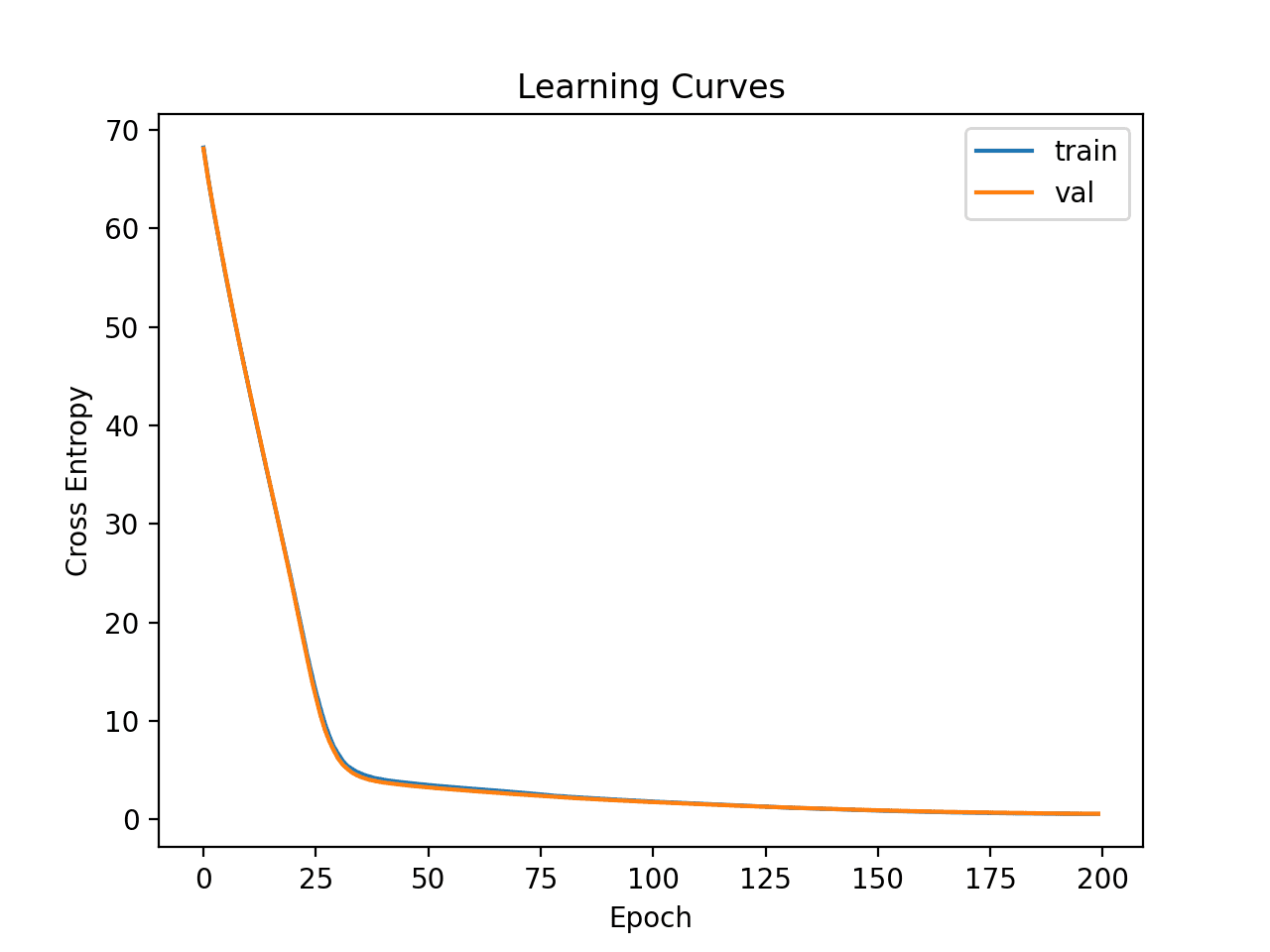
Line plots of the loss on the train and test sets are then created.
We can see that the model quickly finds a good fit on the dataset and does not appear to be over or underfitting.
Learning Curves of Simple Multilayer Perceptron on Cancer Survival Dataset
Now that we have some idea of the learning dynamics for a simple MLP model on the dataset, we can look at developing a more robust evaluation of model performance on the dataset.
Robust Model Evaluation
The k-fold cross-validation procedure can provide a more reliable estimate of MLP performance, although it can be very slow.
This is because k models must be fit and evaluated. This is not a problem when the dataset size is small, such as the cancer survival dataset.
We can use the StratifiedKFold class and enumerate each fold manually, fit the model, evaluate it, and then report the mean of the evaluation scores at the end of the procedure.
We can use this framework to develop a reliable estimate of MLP model performance with our base configuration, and even with a range of different data preparations, model architectures, and learning configurations.
It is important that we first developed an understanding of the learning dynamics of the model on the dataset in the previous section before using k-fold cross-validation to estimate the performance. If we started to tune the model directly, we might get good results, but if not, we might have no idea of why, e.g. that the model was over or under fitting.
If we make large changes to the model again, it is a good idea to go back and confirm that the model is converging appropriately.
The complete example of this framework to evaluate the base MLP model from the previous section is listed below.
1
2
3
4
5
6
7
8
9
10
11
12
13
14
15
16
17
18
19
20
21
22
23
24
25
26
27
28
29
30
31
32
33
34
35
36
37
38
39
40
41
42
43
44
# k-fold cross-validation of base model for the haberman dataset
from numpy import mean
from numpy import std
from pandas import read_csv
from sklearn.model_selection import StratifiedKFold
Running the example reports the model performance each iteration of the evaluation procedure and reports the mean and standard deviation of classification accuracy at the end of the run.
Kick-start your project with my new book Data Preparation for Machine Learning, including step-by-step tutorials and the Python source code files for all examples.
In this case, we can see that the MLP model achieved a mean accuracy of about 75.2 percent, which is pretty close to our rough estimate in the previous section.
This confirms our expectation that the base model configuration may work better than a naive model for this dataset
1
2
3
4
5
6
7
8
9
10
11
>0.742
>0.774
>0.774
>0.806
>0.742
>0.710
>0.767
>0.800
>0.767
>0.633
Mean Accuracy: 0.752 (0.048)
Is this a good result?
In fact, this is a challenging classification problem and achieving a score above about 74.5% is good.
Next, let’s look at how we might fit a final model and use it to make predictions.
Final Model and Make Predictions
Once we choose a model configuration, we can train a final model on all available data and use it to make predictions on new data.
In this case, we will use the model with dropout and a small batch size as our final model.
We can prepare the data and fit the model as before, although on the entire dataset instead of a training subset of the dataset.
We can then use this model to make predictions on new data.
First, we can define a row of new data.
1
2
3
...
# define a row of new data
row=[30,64,1]
Note: I took this row from the first row of the dataset and the expected label is a ‘1’.
We can then make a prediction.
1
2
3
...
# make prediction
yhat=model.predict_classes([row])
Then invert the transform on the prediction, so we can use or interpret the result in the correct label (which is just an integer for this dataset).
1
2
3
...
# invert transform to get label for class
yhat=le.inverse_transform(yhat)
And in this case, we will simply report the prediction.
1
2
3
...
# report prediction
print('Predicted: %s'%(yhat[0]))
Tying this all together, the complete example of fitting a final model for the haberman dataset and using it to make a prediction on new data is listed below.
1
2
3
4
5
6
7
8
9
10
11
12
13
14
15
16
17
18
19
20
21
22
23
24
25
26
27
28
29
30
31
32
33
34
35
# fit a final model and make predictions on new data for the haberman dataset
Running the example fits the model on the entire dataset and makes a prediction for a single row of new data.
Kick-start your project with my new book Data Preparation for Machine Learning, including step-by-step tutorials and the Python source code files for all examples.
In this case, we can see that the model predicted a “1” label for the input row.
1
Predicted: 1
Further Reading
This section provides more resources on the topic if you are looking to go deeper.
Hi Jason. I am confused about this frase “any model that achieves an accuracy less than about 73.5% does not have skill on this dataset”. In the ROC AUC article you said that accuracy can be overly optimistic on the imbalanced dataset.
For this model (Dense(10)) you have accuracy 76.5% but F1 score = 0.0 – does that means that model have no skill?
I’m asking because when I apply SMOTE accuracy drops to 71.6% but F1 increases 0.57. Now I’m confused – does the model has skill now? Which parameter is more important?
Upd. I plotted the chart of F1 and noticed that it depends on the regularizer.
If L2 >= 0.05 F1 fluctuates a lot. It reaches it’s maximum ~0.2 in about 50-70 epochs and drops.
If L2 < 0.05 F1 grows steadily and It reaches it's maximum ~0.5 in about 250 epochs
If L2 < 0.003 F1 grows fast reaches it's maximum ~0.5 in about 50 epochs but then overfitting happens
So – best results without SMOTE on CV split 70/30 (using my custom F1 callback):
2 layers Dense(18) L2 = 0.008
Accuracy = 79.35%
ROC AUC = 0.744
Recall AUC = 0.514
F1 score = 0.558
about this issue on F1 and accuracy: we might be better off and check out the conf matrix and see how much FP or FN we got in the end…and let’s say that the major cost to avoid in medical domain scenario like this is avoid FN : )
Thanks Jason. Training on this dataset is so complicated – I had to read many articles and experiment a lot to get some results.
Now I’m puzzled on how to interpret them:
I split data 70/30 and let’s say I got
Accuracy=75% F1=0.489 on CV (X_test, y_test).
Then I run predictions on a whole dataset (X,y) and it’s better: Accuracy=78.4% F1=0.535.
But for a different regularizer (L2 = 0.007) situation is opposite:
Accuracy=80.39% F1=0.583 on CV dataset (X_test, y_test)
Accuracy=77.43% F1=0.507 on a whole dataset (X,y)
Numbers on a whole dataset should take priority?
What’s the best score that was ever achieved on this dataset?
Hello Diviya…You may be working on a regression problem and achieve zero prediction errors.
Alternately, you may be working on a classification problem and achieve 100% accuracy.
This is unusual and there are many possible reasons for this, including:
You are evaluating model performance on the training set by accident.
Your hold out dataset (train or validation) is too small or unrepresentative.
You have introduced a bug into your code and it is doing something different from what you expect.
Your prediction problem is easy or trivial and may not require machine learning.
The most common reason is that your hold out dataset is too small or not representative of the broader problem.
This can be addressed by:
Using k-fold cross-validation to estimate model performance instead of a train/test split.
Gather more data.
Use a different split of data for train and test, such as 50/50.
Jason, I discovered your article with some delay but I read it with great interest because it reflects a research project of mine from over 30 years ago. I’ve been trying to get your source codes to work using data different from the Haberman dataset. The Haberman data in fact it has a big flaw, the date of the surgical operation has generally very little relevance on survival. I was wondering how one can modify the python sources to examine, say, more than n. 3 variables.
Your code gives me an error because the “model.predict_classes()” is deprecated since 2021, evidently after you wrote this article.
I rewrote it like this and it seems to work:
from sklearn.metrics import accuracy_score
yhat = np.argmax(model.predict(X_test), axis=-1)
# ‘yhat’ is the ‘prediction’ (I hope so)
# evaluate predictions
score = accuracy_score(y_test, yhat)
print(‘\nAccuracy: %.3f’ % score)
I am a medical doctor and not a professional programmer, you must therefore excuse me.
On chapter “Neural Network Learning Dynamics” I achieved only 0.73 Accuracy, since the I’m using a different version of TF I don’t now if anything in my code has changed which for instance affected the accuracy, for it to work I had to adjust the Test Prediction to something “yhat = np.argmax(model.predict(X_test), axis=1)” I don’t if it affects the accuracy or not. I’ve been reading the TF documentation and I don’t find any clues.


Hi Jason. I am confused about this frase “any model that achieves an accuracy less than about 73.5% does not have skill on this dataset”. In the ROC AUC article you said that accuracy can be overly optimistic on the imbalanced dataset.
For this model (Dense(10)) you have accuracy 76.5% but F1 score = 0.0 – does that means that model have no skill?
I’m asking because when I apply SMOTE accuracy drops to 71.6% but F1 increases 0.57. Now I’m confused – does the model has skill now? Which parameter is more important?
Upd. F1 is not always 0.0 after 200 epochs. Sometimes it’s 0.127
Upd. I plotted the chart of F1 and noticed that it depends on the regularizer.
If L2 >= 0.05 F1 fluctuates a lot. It reaches it’s maximum ~0.2 in about 50-70 epochs and drops.
If L2 < 0.05 F1 grows steadily and It reaches it's maximum ~0.5 in about 250 epochs
If L2 < 0.003 F1 grows fast reaches it's maximum ~0.5 in about 50 epochs but then overfitting happens
So – best results without SMOTE on CV split 70/30 (using my custom F1 callback):
2 layers Dense(18) L2 = 0.008
Accuracy = 79.35%
ROC AUC = 0.744
Recall AUC = 0.514
F1 score = 0.558
Yes, F1 would be a better metric for this dataset.
about this issue on F1 and accuracy: we might be better off and check out the conf matrix and see how much FP or FN we got in the end…and let’s say that the major cost to avoid in medical domain scenario like this is avoid FN : )
Thanks Jason. Training on this dataset is so complicated – I had to read many articles and experiment a lot to get some results.
Now I’m puzzled on how to interpret them:
I split data 70/30 and let’s say I got
Accuracy=75% F1=0.489 on CV (X_test, y_test).
Then I run predictions on a whole dataset (X,y) and it’s better: Accuracy=78.4% F1=0.535.
But for a different regularizer (L2 = 0.007) situation is opposite:
Accuracy=80.39% F1=0.583 on CV dataset (X_test, y_test)
Accuracy=77.43% F1=0.507 on a whole dataset (X,y)
Numbers on a whole dataset should take priority?
What’s the best score that was ever achieved on this dataset?
I would recommend selecting one metric, and one robust test harness like repeated stratified k-fold cv.
sir how to resolve following error i already have keras installed
No module named ‘keras.cross_validation’
I think there’s an error in your code.
Im getting 0 for my accuracy.. Can I know what can be the reason?
Hello Diviya…You may be working on a regression problem and achieve zero prediction errors.
Alternately, you may be working on a classification problem and achieve 100% accuracy.
This is unusual and there are many possible reasons for this, including:
You are evaluating model performance on the training set by accident.
Your hold out dataset (train or validation) is too small or unrepresentative.
You have introduced a bug into your code and it is doing something different from what you expect.
Your prediction problem is easy or trivial and may not require machine learning.
The most common reason is that your hold out dataset is too small or not representative of the broader problem.
This can be addressed by:
Using k-fold cross-validation to estimate model performance instead of a train/test split.
Gather more data.
Use a different split of data for train and test, such as 50/50.
In the text it is mentioned the addition of dropout, but I don’t see it in the code
Jason, I discovered your article with some delay but I read it with great interest because it reflects a research project of mine from over 30 years ago. I’ve been trying to get your source codes to work using data different from the Haberman dataset. The Haberman data in fact it has a big flaw, the date of the surgical operation has generally very little relevance on survival. I was wondering how one can modify the python sources to examine, say, more than n. 3 variables.
Your code gives me an error because the “model.predict_classes()” is deprecated since 2021, evidently after you wrote this article.
I rewrote it like this and it seems to work:
from sklearn.metrics import accuracy_score
yhat = np.argmax(model.predict(X_test), axis=-1)
# ‘yhat’ is the ‘prediction’ (I hope so)
# evaluate predictions
score = accuracy_score(y_test, yhat)
print(‘\nAccuracy: %.3f’ % score)
I am a medical doctor and not a professional programmer, you must therefore excuse me.
Hi Daniel…Thank you for your feedback! Keep up the great work!
The following location is a great place to start to build your machine learning knowledge:
https://machinelearningmastery.com/start-here/
Hi James,
On chapter “Neural Network Learning Dynamics” I achieved only 0.73 Accuracy, since the I’m using a different version of TF I don’t now if anything in my code has changed which for instance affected the accuracy, for it to work I had to adjust the Test Prediction to something “yhat = np.argmax(model.predict(X_test), axis=1)” I don’t if it affects the accuracy or not. I’ve been reading the TF documentation and I don’t find any clues.
Hi Alcides…You may want to try your code in Google Colab to determine if there are any version differences.
Hi James,
I Colab I’ve Tensoflow version 2.12 and in my machine is 2.13.0-rc.
Running exactly the same code, I got the same result in terms of accuracy. Maybe, I’m doing something wrong.