Imbalanced Classification with the Adult Income Dataset

Many binary classification tasks do not have an equal number of examples from each class, e.g. the class distribution is skewed or imbalanced.

A popular example is the adult income dataset that involves predicting personal income levels as above or below $50,000 per year based on personal details such as relationship and education level. There are many more cases of incomes less than $50K than above $50K, although the skew is not severe.

This means that techniques for imbalanced classification can be used whilst model performance can still be reported using classification accuracy, as is used with balanced classification problems.

In this tutorial, you will discover how to develop and evaluate a model for the imbalanced adult income classification dataset.

After completing this tutorial, you will know:

• How to load and explore the dataset and generate ideas for data preparation and model selection.
• How to systematically evaluate a suite of machine learning models with a robust test harness.
• How to fit a final model and use it to predict class labels for specific cases.

Kick-start your project with my new book Imbalanced Classification with Python, including step-by-step tutorials and the Python source code files for all examples.

Let’s get started.

Develop an Imbalanced Classification Model to Predict Income
Photo by Kirt Edblom, some rights reserved.

Tutorial Overview

This tutorial is divided into five parts; they are:

1. Adult Income Dataset
2. Explore the Dataset
3. Model Test and Baseline Result
4. Evaluate Models
5. Make Prediction on New Data

Adult Income Dataset

In this project, we will use a standard imbalanced machine learning dataset referred to as the “Adult Income” or simply the “adult” dataset.

The dataset is credited to Ronny Kohavi and Barry Becker and was drawn from the 1994 United States Census Bureau data and involves using personal details such as education level to predict whether an individual will earn more or less than $50,000 per year.

The Adult dataset is from the Census Bureau and the task is to predict whether a given adult makes more than $50,000 a year based attributes such as education, hours of work per week, etc..

— Scaling Up The Accuracy Of Naive-bayes Classifiers: A Decision-tree Hybrid, 1996.

The dataset provides 14 input variables that are a mixture of categorical, ordinal, and numerical data types. The complete list of variables is as follows:

• Age.
• Workclass.
• Final Weight.
• Education.
• Education Number of Years.
• Marital-status.
• Occupation.
• Relationship.
• Race.
• Sex.
• Capital-gain.
• Capital-loss.
• Hours-per-week.
• Native-country.

The dataset contains missing values that are marked with a question mark character (?).

There are a total of 48,842 rows of data, and 3,620 with missing values, leaving 45,222 complete rows.

There are two class values ‘>50K‘ and ‘<=50K‘, meaning it is a binary classification task. The classes are imbalanced, with a skew toward the ‘<=50K‘ class label.

• ‘>50K’: majority class, approximately 25%.
• ‘<=50K’: minority class, approximately 75%.

Given that the class imbalance is not severe and that both class labels are equally important, it is common to use classification accuracy or classification error to report model performance on this dataset.

Using predefined train and test sets, reported good classification error is approximately 14 percent or a classification accuracy of about 86 percent. This might provide a target to aim for when working on this dataset.

Next, let’s take a closer look at the data.

Explore the Dataset

The Adult dataset is a widely used standard machine learning dataset, used to explore and demonstrate many machine learning algorithms, both generally and those designed specifically for imbalanced classification.

First, download the dataset and save it in your current working directory with the name “adult-all.csv”

• Download Adult Dataset (adult-all.csv)

Review the contents of the file.

The first few lines of the file should look as follows:

We can see that the input variables are a mixture of numerical and categorical or ordinal data types, where the non-numerical columns are represented using strings. At a minimum, the categorical variables will need to be ordinal or one-hot encoded.

We can also see that the target variable is represented using strings. This column will need to be label encoded with 0 for the majority class and 1 for the minority class, as is the custom for binary imbalanced classification tasks.

Missing values are marked with a ‘?‘ character. These values will need to be imputed, or given the small number of examples, these rows could be deleted from the dataset.

The dataset can be loaded as a DataFrame using the read_csv() Pandas function, specifying the filename, that there is no header line, and that strings like ‘ ?‘ should be parsed as NaN (missing) values.

Once loaded, we can remove the rows that contain one or more missing values.

We can summarize the number of rows and columns by printing the shape of the DataFrame.

We can also summarize the number of examples in each class using the Counter object.

Tying this together, the complete example of loading and summarizing the dataset is listed below.

Running the example first loads the dataset and confirms the number of rows and columns, that is 45,222 rows without missing values and 14 input variables and one target variable.

The class distribution is then summarized, confirming a modest class imbalance with approximately 75 percent for the majority class (<=50K) and approximately 25 percent for the minority class (>50K).

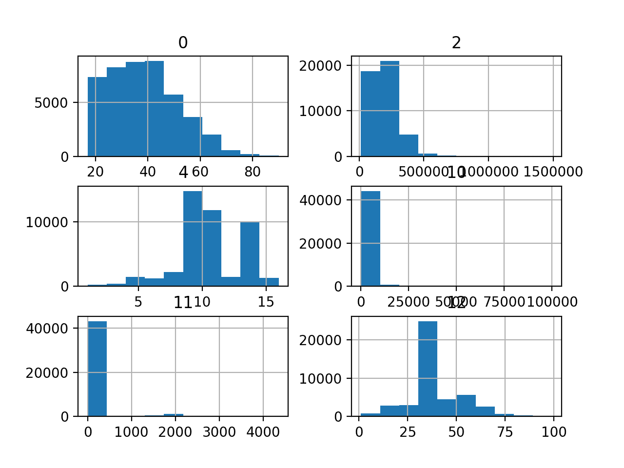
We can also take a look at the distribution of the numerical input variables by creating a histogram for each.

First, we can select the columns with numeric variables by calling the select_dtypes() function on the DataFrame. We can then select just those columns from the DataFrame.

We can then create histograms of each numeric input variable. The complete example is listed below.

Running the example creates the figure with one histogram subplot for each of the six input variables in the dataset. The title of each subplot indicates the column number in the DataFrame (e.g. zero-offset).

We can see many different distributions, some with Gaussian-like distributions, others with seemingly exponential or discrete distributions. We can also see that they all appear to have a very different scale.

Depending on the choice of modeling algorithms, we would expect scaling the distributions to the same range to be useful, and perhaps the use of some power transforms.

Histogram of Numeric Variables in the Adult Imbalanced Classification Dataset

Now that we have reviewed the dataset, let’s look at developing a test harness for evaluating candidate models.

Model Test and Baseline Result

We will evaluate candidate models using repeated stratified k-fold cross-validation.

The k-fold cross-validation procedure provides a good general estimate of model performance that is not too optimistically biased, at least compared to a single train-test split. We will use k=10, meaning each fold will contain about 45,222/10, or about 4,522 examples.

Stratified means that each fold will contain the same mixture of examples by class, that is about 75 percent to 25 percent for the majority and minority classes respectively. Repeated means that the evaluation process will be performed multiple times to help avoid fluke results and better capture the variance of the chosen model. We will use three repeats.

This means a single model will be fit and evaluated 10 * 3 or 30 times and the mean and standard deviation of these runs will be reported.

This can be achieved using the RepeatedStratifiedKFold scikit-learn class.

We will predict a class label for each example and measure model performance using classification accuracy.

The evaluate_model() function below will take the loaded dataset and a defined model and will evaluate it using repeated stratified k-fold cross-validation, then return a list of accuracy scores that can later be summarized.

We can define a function to load the dataset and label encode the target column.

We will also return a list of categorical and numeric columns in case we decide to transform them later when fitting models.

Finally, we can evaluate a baseline model on the dataset using this test harness.

When using classification accuracy, a naive model will predict the majority class for all cases. This provides a baseline in model performance on this problem by which all other models can be compared.

This can be achieved using the DummyClassifier class from the scikit-learn library and setting the “strategy” argument to ‘most_frequent‘.

Once the model is evaluated, we can report the mean and standard deviation of the accuracy scores directly.

Tying this together, the complete example of loading the Adult dataset, evaluating a baseline model, and reporting the performance is listed below.

Running the example first loads and summarizes the dataset.

We can see that we have the correct number of rows loaded. Importantly, we can see that the class labels have the correct mapping to integers, with 0 for the majority class and 1 for the minority class, customary for imbalanced binary classification dataset.

Next, the average classification accuracy score is reported.

In this case, we can see that the baseline algorithm achieves an accuracy of about 75.2%. This score provides a lower limit on model skill; any model that achieves an average accuracy above about 75.2% has skill, whereas models that achieve a score below this value do not have skill on this dataset.

Now that we have a test harness and a baseline in performance, we can begin to evaluate some models on this dataset.

Evaluate Models

In this section, we will evaluate a suite of different techniques on the dataset using the test harness developed in the previous section.

The goal is to both demonstrate how to work through the problem systematically and to demonstrate the capability of some techniques designed for imbalanced classification problems.

The reported performance is good, but not highly optimized (e.g. hyperparameters are not tuned).

Can you do better? If you can achieve better classification accuracy performance using the same test harness, I’d love to hear about it. Let me know in the comments below.

Evaluate Machine Learning Algorithms

Let’s start by evaluating a mixture of machine learning models on the dataset.

It can be a good idea to spot check a suite of different nonlinear algorithms on a dataset to quickly flush out what works well and deserves further attention, and what doesn’t.

We will evaluate the following machine learning models on the adult dataset:

• Decision Tree (CART)
• Support Vector Machine (SVM)
• Bagged Decision Trees (BAG)
• Random Forest (RF)
• Gradient Boosting Machine (GBM)

We will use mostly default model hyperparameters, with the exception of the number of trees in the ensemble algorithms, which we will set to a reasonable default of 100.

We will define each model in turn and add them to a list so that we can evaluate them sequentially. The get_models() function below defines the list of models for evaluation, as well as a list of model short names for plotting the results later.

We can then enumerate the list of models in turn and evaluate each, storing the scores for later evaluation.

We will one-hot encode the categorical input variables using a OneHotEncoder, and we will normalize the numerical input variables using the MinMaxScaler. These operations must be performed within each train/test split during the cross-validation process, where the encoding and scaling operations are fit on the training set and applied to the train and test sets.

An easy way to implement this is to use a Pipeline where the first step is a ColumnTransformer that applies a OneHotEncoder to just the categorical variables, and a MinMaxScaler to just the numerical input variables. To achieve this, we need a list of the column indices for categorical and numerical input variables.

The load_dataset() function we defined in the previous section loads and returns both the dataset and lists of columns that have categorical and numerical data types. This can be used to prepare a Pipeline to wrap each model prior to evaluating it. First, the ColumnTransformer is defined, which specifies what transform to apply to each type of column, then this is used as the first step in a Pipeline that ends with the specific model that will be fit and evaluated.

We can summarize the mean accuracy for each algorithm, this will help to directly compare algorithms.

At the end of the run, we will create a separate box and whisker plot for each algorithm’s sample of results. These plots will use the same y-axis scale so we can compare the distribution of results directly.

Tying this all together, the complete example of evaluation a suite of machine learning algorithms on the adult imbalanced dataset is listed below.

Running the example evaluates each algorithm in turn and reports the mean and standard deviation classification accuracy.

Note: Your results may vary given the stochastic nature of the algorithm or evaluation procedure, or differences in numerical precision. Consider running the example a few times and compare the average outcome.

What scores did you get?
Post your results in the comments below.

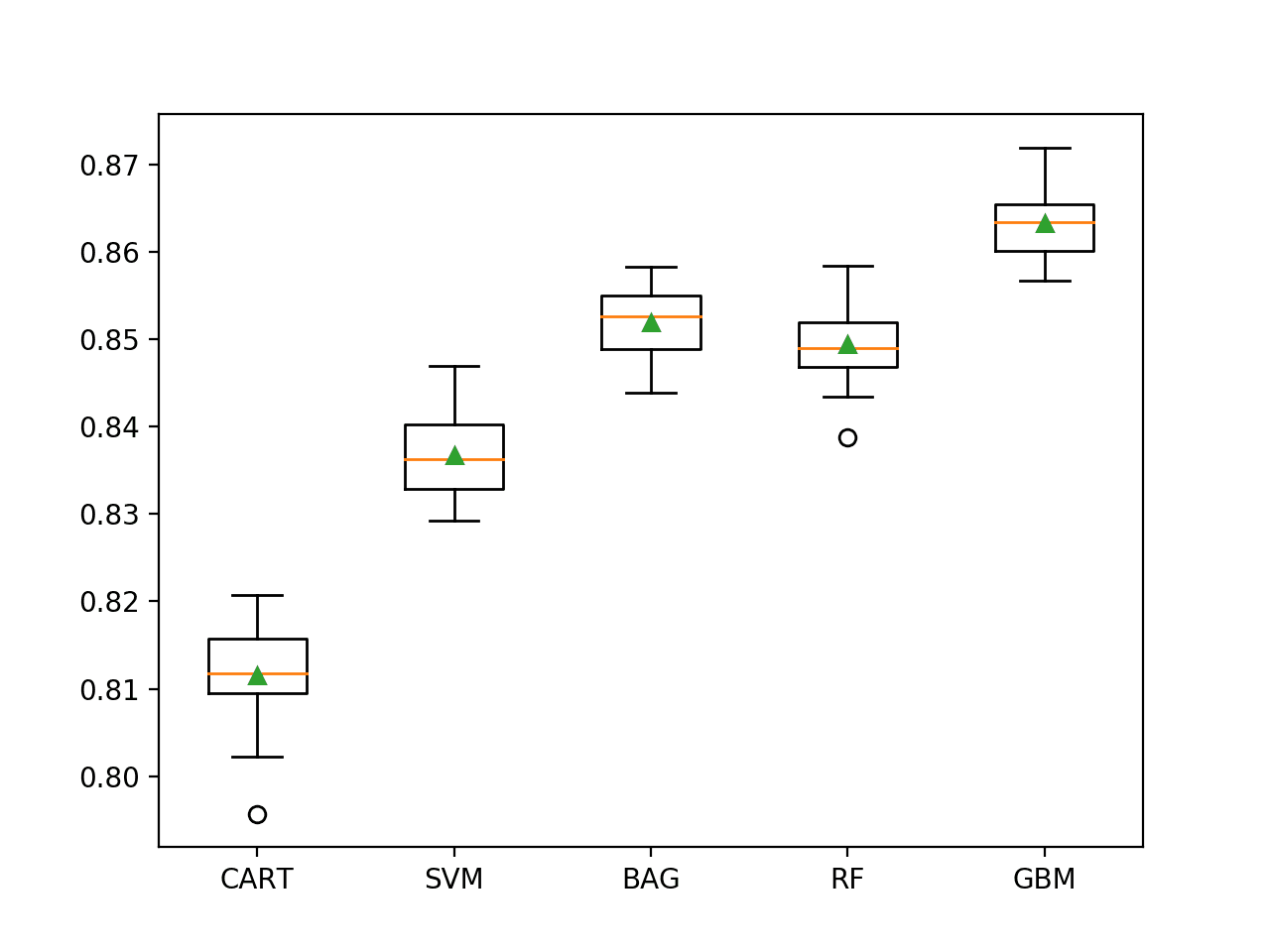
In this case, we can see that all of the chosen algorithms are skillful, achieving a classification accuracy above 75.2%. We can see that the ensemble decision tree algorithms perform the best with perhaps stochastic gradient boosting performing the best with a classification accuracy of about 86.3%.

This is slightly better than the result reported in the original paper, albeit with a different model evaluation procedure.

A figure is created showing one box and whisker plot for each algorithm’s sample of results. The box shows the middle 50 percent of the data, the orange line in the middle of each box shows the median of the sample, and the green triangle in each box shows the mean of the sample.

We can see that the distribution of scores for each algorithm appears to be above the baseline of about 75%, perhaps with a few outliers (circles on the plot). The distribution for each algorithm appears compact, with the median and mean aligning, suggesting the models are quite stable on this dataset and scores do not form a skewed distribution.

This highlights that it is not just the central tendency of the model performance that it is important, but also the spread and even worst-case result that should be considered. Especially with a limited number of examples of the minority class.

Box and Whisker Plot of Machine Learning Models on the Imbalanced Adult Dataset

Make Prediction on New Data

In this section, we can fit a final model and use it to make predictions on single rows of data.

We will use the GradientBoostingClassifier model as our final model that achieved a classification accuracy of about 86.3%. Fitting the final model involves defining the ColumnTransformer to encode the categorical variables and scale the numerical variables, then construct a Pipeline to perform these transforms on the training set prior to fitting the model.

The Pipeline can then be used to make predictions on new data directly, and will automatically encode and scale new data using the same operations as were performed on the training dataset.

First, we can define the model as a pipeline.

Once defined, we can fit it on the entire training dataset.

Once fit, we can use it to make predictions for new data by calling the predict() function. This will return the class label of 0 for “<=50K”, or 1 for “>50K”.

Importantly, we must use the ColumnTransformer within the Pipeline to correctly prepare new data using the same transforms.

For example:

To demonstrate this, we can use the fit model to make some predictions of labels for a few cases where we know the outcome.

The complete example is listed below.

Running the example first fits the model on the entire training dataset.

Then the fit model used to predict the label of <=50K cases is chosen from the dataset file. We can see that all cases are correctly predicted. Then some >50K cases are used as input to the model and the label is predicted. As we might have hoped, the correct labels are predicted.

Further Reading

This section provides more resources on the topic if you are looking to go deeper.

Papers

• Scaling Up The Accuracy Of Naive-bayes Classifiers: A Decision-tree Hybrid, 1996.

APIs

• pandas.DataFrame.select_dtypes API.
• sklearn.model_selection.RepeatedStratifiedKFold API.
• sklearn.dummy.DummyClassifier API.

Dataset

• Adult Dataset CSV.
• Adult Dataset Description.
• Adult Dataset, UCI Machine Learning Repository.

Summary

In this tutorial, you discovered how to develop and evaluate a model for the imbalanced adult income classification dataset.

Specifically, you learned:

• How to load and explore the dataset and generate ideas for data preparation and model selection.
• How to systematically evaluate a suite of machine learning models with a robust test harness.
• How to fit a final model and use it to predict class labels for specific cases.

Do you have any questions?
Ask your questions in the comments below and I will do my best to answer.

Get a Handle on Imbalanced Classification!

Develop Imbalanced Learning Models in Minutes

...with just a few lines of python code

Discover how in my new Ebook:
Imbalanced Classification with Python

It provides self-study tutorials and end-to-end projects on:
Performance Metrics, Undersampling Methods, SMOTE, Threshold Moving, Probability Calibration, Cost-Sensitive Algorithms
and much more...

Bring Imbalanced Classification Methods to Your Machine Learning Projects

See What's Inside