Most imbalanced classification problems involve two classes: a negative case with the majority of examples and a positive case with a minority of examples.
Two diagnostic tools that help in the interpretation of binary (two-class) classification predictive models are ROC Curves and Precision-Recall curves.
Plots from the curves can be created and used to understand the trade-off in performance for different threshold values when interpreting probabilistic predictions. Each plot can also be summarized with an area under the curve score that can be used to directly compare classification models.
In this tutorial, you will discover ROC Curves and Precision-Recall Curves for imbalanced classification.
After completing this tutorial, you will know:
ROC Curves and Precision-Recall Curves provide a diagnostic tool for binary classification models.
ROC AUC and Precision-Recall AUC provide scores that summarize the curves and can be used to compare classifiers.
ROC Curves and ROC AUC can be optimistic on severely imbalanced classification problems with few samples of the minority class.
Kick-start your project with my new book Imbalanced Classification with Python, including step-by-step tutorials and the Python source code files for all examples.
Let’s get started.
ROC Curves and Precision-Recall Curves for Imbalanced Classification Photo by Nicholas A. Tonelli, some rights reserved.
Tutorial Overview
This tutorial is divided into four parts; they are:
Review of the Confusion Matrix
ROC Curves and ROC AUC
Precision-Recall Curves and AUC
ROC and Precision-Recall Curves With a Severe Imbalance
Review of the Confusion Matrix
Before we dive into ROC Curves and PR Curves, it is important to review the confusion matrix.
For imbalanced classification problems, the majority class is typically referred to as the negative outcome (e.g. such as “no change” or “negative test result“), and the minority class is typically referred to as the positive outcome (e.g. “change” or “positive test result“).
The confusion matrix provides more insight into not only the performance of a predictive model, but also which classes are being predicted correctly, which incorrectly, and what type of errors are being made.
The simplest confusion matrix is for a two-class classification problem, with negative (class 0) and positive (class 1) classes.
In this type of confusion matrix, each cell in the table has a specific and well-understood name, summarized as follows:
1
2
3
| Positive Prediction | Negative Prediction
Positive Class | True Positive (TP) | False Negative (FN)
Negative Class | False Positive (FP) | True Negative (TN)
The metrics that make up the ROC curve and the precision-recall curve are defined in terms of the cells in the confusion matrix.
Now that we have brushed up on the confusion matrix, let’s take a closer look at the ROC Curves metric.
Want to Get Started With Imbalance Classification?
Take my free 7-day email crash course now (with sample code).
Click to sign-up and also get a free PDF Ebook version of the course.
ROC Curves and ROC AUC
An ROC curve (or receiver operating characteristic curve) is a plot that summarizes the performance of a binary classification model on the positive class.
The x-axis indicates the False Positive Rate and the y-axis indicates the True Positive Rate.
ROC Curve: Plot of False Positive Rate (x) vs. True Positive Rate (y).
The true positive rate is a fraction calculated as the total number of true positive predictions divided by the sum of the true positives and the false negatives (e.g. all examples in the positive class). The true positive rate is referred to as the sensitivity or the recall.
The false positive rate is calculated as the total number of false positive predictions divided by the sum of the false positives and true negatives (e.g. all examples in the negative class).
We can think of the plot as the fraction of correct predictions for the positive class (y-axis) versus the fraction of errors for the negative class (x-axis).
Ideally, we want the fraction of correct positive class predictions to be 1 (top of the plot) and the fraction of incorrect negative class predictions to be 0 (left of the plot). This highlights that the best possible classifier that achieves perfect skill is the top-left of the plot (coordinate 0,1).
Perfect Skill: A point in the top left of the plot.
The threshold is applied to the cut-off point in probability between the positive and negative classes, which by default for any classifier would be set at 0.5, halfway between each outcome (0 and 1).
A trade-off exists between the TruePositiveRate and FalsePositiveRate, such that changing the threshold of classification will change the balance of predictions towards improving the TruePositiveRate at the expense of FalsePositiveRate, or the reverse case.
By evaluating the true positive and false positives for different threshold values, a curve can be constructed that stretches from the bottom left to top right and bows toward the top left. This curve is called the ROC curve.
A classifier that has no discriminative power between positive and negative classes will form a diagonal line between a False Positive Rate of 0 and a True Positive Rate of 0 (coordinate (0,0) or predict all negative class) to a False Positive Rate of 1 and a True Positive Rate of 1 (coordinate (1,1) or predict all positive class). Models represented by points below this line have worse than no skill.
The curve provides a convenient diagnostic tool to investigate one classifier with different threshold values and the effect on the TruePositiveRate and FalsePositiveRate. One might choose a threshold in order to bias the predictive behavior of a classification model.
It is a popular diagnostic tool for classifiers on balanced and imbalanced binary prediction problems alike because it is not biased to the majority or minority class.
ROC analysis does not have any bias toward models that perform well on the minority class at the expense of the majority class—a property that is quite attractive when dealing with imbalanced data.
The function takes both the true outcomes (0,1) from the test set and the predicted probabilities for the 1 class. The function returns the false positive rates for each threshold, true positive rates for each threshold and thresholds.
1
2
3
...
# calculate roc curve
fpr,tpr,thresholds=roc_curve(testy,pos_probs)
Most scikit-learn models can predict probabilities by calling the predict_proba() function.
This will return the probabilities for each class, for each sample in a test set, e.g. two numbers for each of the two classes in a binary classification problem. The probabilities for the positive class can be retrieved as the second column in this array of probabilities.
1
2
3
4
5
...
# predict probabilities
yhat=model.predict_proba(testX)
# retrieve just the probabilities for the positive class
pos_probs=yhat[:,1]
We can demonstrate this on a synthetic dataset and plot the ROC curve for a no skill classifier and a Logistic Regression model.
The make_classification() function can be used to create synthetic classification problems. In this case, we will create 1,000 examples for a binary classification problem (about 500 examples per class). We will then split the dataset into a train and test sets of equal size in order to fit and evaluate the model.
A Logistic Regression model is a good model for demonstration because the predicted probabilities are well-calibrated, as opposed to other machine learning models that are not developed around a probabilistic model, in which case their probabilities may need to be calibrated first (e.g. an SVM).
1
2
3
4
...
# fit a model
model=LogisticRegression(solver='lbfgs')
model.fit(trainX,trainy)
The complete example is listed below.
1
2
3
4
5
6
7
8
9
10
11
12
13
14
15
16
17
18
19
20
21
22
23
24
25
26
27
28
29
30
# example of a roc curve for a predictive model
from sklearn.datasets import make_classification
from sklearn.linear_model import LogisticRegression
from sklearn.model_selection import train_test_split
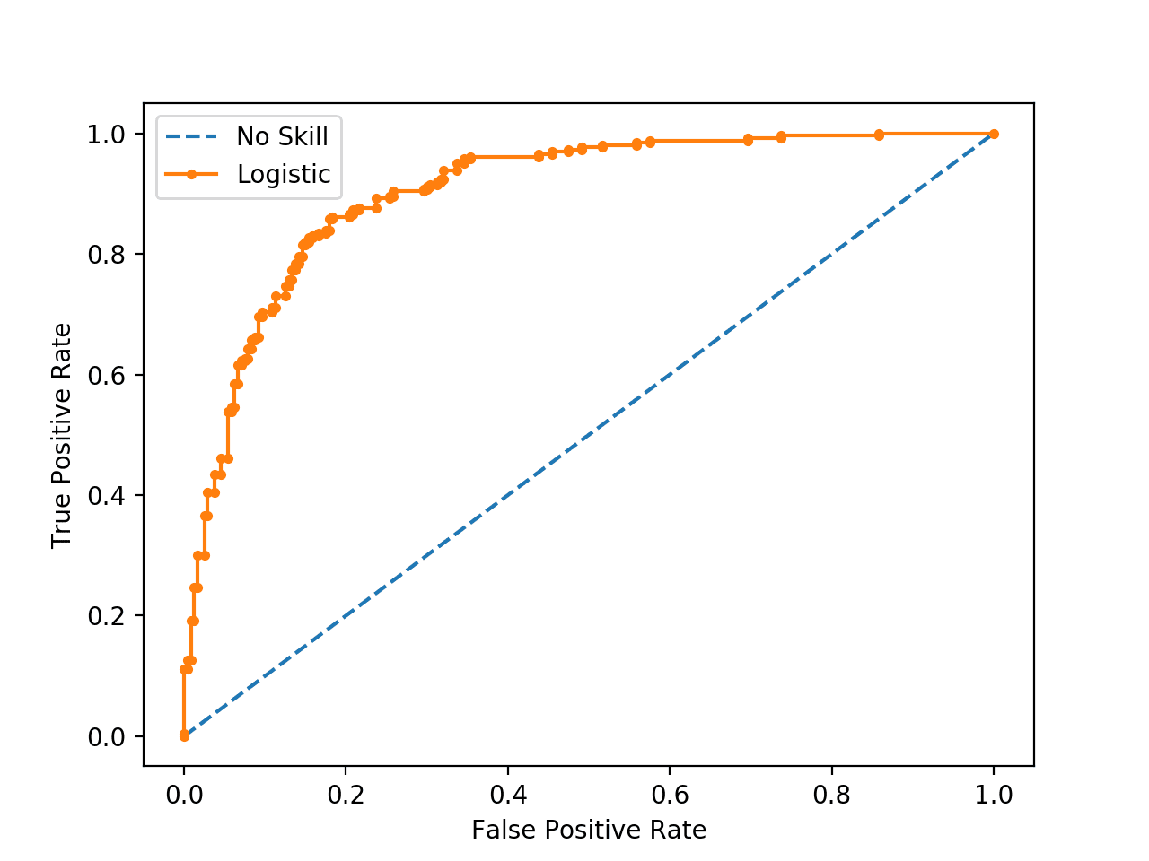
Running the example creates the synthetic dataset, splits into train and test sets, then fits a Logistic Regression model on the training dataset and uses it to make a prediction on the test set.
The ROC Curve for the Logistic Regression model is shown (orange with dots). A no skill classifier as a diagonal line (blue with dashes).
ROC Curve of a Logistic Regression Model and a No Skill Classifier
Now that we have seen the ROC Curve, let’s take a closer look at the ROC area under curve score.
ROC Area Under Curve (AUC) Score
Although the ROC Curve is a helpful diagnostic tool, it can be challenging to compare two or more classifiers based on their curves.
Instead, the area under the curve can be calculated to give a single score for a classifier model across all threshold values. This is called the ROC area under curve or ROC AUC or sometimes ROCAUC.
The score is a value between 0.0 and 1.0 for a perfect classifier.
AUCROC can be interpreted as the probability that the scores given by a classifier will rank a randomly chosen positive instance higher than a randomly chosen negative one.
This single score can be used to compare binary classifier models directly. As such, this score might be the most commonly used for comparing classification models for imbalanced problems.
The most common metric involves receiver operation characteristics (ROC) analysis, and the area under the ROC curve (AUC).
Like the roc_curve() function, the AUC function takes both the true outcomes (0,1) from the test set and the predicted probabilities for the positive class.
1
2
3
...
# calculate roc auc
roc_auc=roc_auc_score(testy,pos_probs)
We can demonstrate this the same synthetic dataset with a Logistic Regression model.
The complete example is listed below.
1
2
3
4
5
6
7
8
9
10
11
12
13
14
15
16
17
18
19
20
21
22
23
24
25
26
# example of a roc auc for a predictive model
from sklearn.datasets import make_classification
from sklearn.dummy import DummyClassifier
from sklearn.linear_model import LogisticRegression
from sklearn.model_selection import train_test_split
# no skill model, stratified random class predictions
model=DummyClassifier(strategy='stratified')
model.fit(trainX,trainy)
yhat=model.predict_proba(testX)
pos_probs=yhat[:,1]
# calculate roc auc
roc_auc=roc_auc_score(testy,pos_probs)
print('No Skill ROC AUC %.3f'%roc_auc)
# skilled model
model=LogisticRegression(solver='lbfgs')
model.fit(trainX,trainy)
yhat=model.predict_proba(testX)
pos_probs=yhat[:,1]
# calculate roc auc
roc_auc=roc_auc_score(testy,pos_probs)
print('Logistic ROC AUC %.3f'%roc_auc)
Running the example creates and splits the synthetic dataset, fits the model, and uses the fit model to predict probabilities on the test dataset.
Note: Your results may vary given the stochastic nature of the algorithm or evaluation procedure, or differences in numerical precision. Consider running the example a few times and compare the average outcome.
In this case, we can see that the ROC AUC for the Logistic Regression model on the synthetic dataset is about 0.903, which is much better than a no skill classifier with a score of about 0.5.
1
2
No Skill ROC AUC 0.509
Logistic ROC AUC 0.903
Although widely used, the ROC AUC is not without problems.
For imbalanced classification with a severe skew and few examples of the minority class, the ROC AUC can be misleading. This is because a small number of correct or incorrect predictions can result in a large change in the ROC Curve or ROC AUC score.
Although ROC graphs are widely used to evaluate classifiers under presence of class imbalance, it has a drawback: under class rarity, that is, when the problem of class imbalance is associated to the presence of a low sample size of minority instances, as the estimates can be unreliable.
The result is a value between 0.0 for no precision and 1.0 for full or perfect precision.
Recall is a metric that quantifies the number of correct positive predictions made out of all positive predictions that could have been made.
It is calculated as the number of true positives divided by the total number of true positives and false negatives (e.g. it is the true positive rate).
A precision-recall curve (or PR Curve) is a plot of the precision (y-axis) and the recall (x-axis) for different probability thresholds.
PR Curve: Plot of Recall (x) vs Precision (y).
A model with perfect skill is depicted as a point at a coordinate of (1,1). A skillful model is represented by a curve that bows towards a coordinate of (1,1). A no-skill classifier will be a horizontal line on the plot with a precision that is proportional to the number of positive examples in the dataset. For a balanced dataset this will be 0.5.
The focus of the PR curve on the minority class makes it an effective diagnostic for imbalanced binary classification models.
Precision-recall curves (PR curves) are recommended for highly skewed domains where ROC curves may provide an excessively optimistic view of the performance.
A precision-recall curve can be calculated in scikit-learn using the precision_recall_curve() function that takes the class labels and predicted probabilities for the minority class and returns the precision, recall, and thresholds.
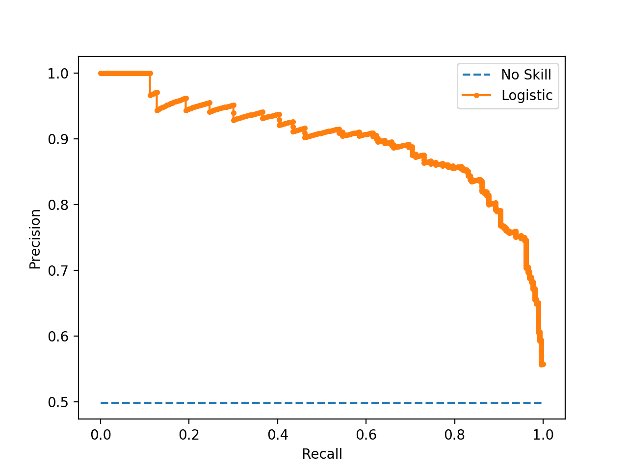
Running the example creates the synthetic dataset, splits into train and test sets, then fits a Logistic Regression model on the training dataset and uses it to make a prediction on the test set.
The Precision-Recall Curve for the Logistic Regression model is shown (orange with dots). A random or baseline classifier is shown as a horizontal line (blue with dashes).
Precision-Recall Curve of a Logistic Regression Model and a No Skill Classifier
Now that we have seen the Precision-Recall Curve, let’s take a closer look at the ROC area under curve score.
Precision-Recall Area Under Curve (AUC) Score
The Precision-Recall AUC is just like the ROC AUC, in that it summarizes the curve with a range of threshold values as a single score.
The score can then be used as a point of comparison between different models on a binary classification problem where a score of 1.0 represents a model with perfect skill.
The Precision-Recall AUC score can be calculated using the auc() function in scikit-learn, taking the precision and recall values as arguments.
1
2
3
...
# calculate the precision-recall auc
auc_score=auc(recall,precision)
Again, we can demonstrate calculating the Precision-Recall AUC for a Logistic Regression on a synthetic dataset.
The complete example is listed below.
1
2
3
4
5
6
7
8
9
10
11
12
13
14
15
16
17
18
19
20
21
22
23
24
25
26
27
28
29
# example of a precision-recall auc for a predictive model
from sklearn.datasets import make_classification
from sklearn.dummy import DummyClassifier
from sklearn.linear_model import LogisticRegression
from sklearn.model_selection import train_test_split
from sklearn.metrics import precision_recall_curve
Running the example creates and splits the synthetic dataset, fits the model, and uses the fit model to predict probabilities on the test dataset.
Note: Your results may vary given the stochastic nature of the algorithm or evaluation procedure, or differences in numerical precision. Consider running the example a few times and compare the average outcome.
In this case, we can see that the Precision-Recall AUC for the Logistic Regression model on the synthetic dataset is about 0.898, which is much better than a no skill classifier that would achieve the score in this case of 0.632.
1
2
No Skill PR AUC: 0.632
Logistic PR AUC: 0.898
ROC and Precision-Recall Curves With a Severe Imbalance
In this section, we will explore the case of using the ROC Curves and Precision-Recall curves with a binary classification problem that has a severe class imbalance.
Firstly, we can use the make_classification() function to create 1,000 examples for a classification problem with about a 1:100 minority to majority class ratio. This can be achieved by setting the “weights” argument and specifying the weighting of generated instances from each class.
We will use a 99 percent and 1 percent weighting with 1,000 total examples, meaning there would be about 990 for class 0 and about 10 for class 1.
We can then split the dataset into training and test sets and ensure that both have the same general class ratio by setting the “stratify” argument on the call to the train_test_split() function and setting it to the array of target variables.
1
2
3
...
# split into train/test sets with same class ratio
Running the example first summarizes the class ratio of the whole dataset, then the ratio for each of the train and test sets, confirming the split of the dataset holds the same ratio.
1
2
3
Dataset: Class0=985, Class1=15
Train: Class0=492, Class1=8
Test: Class0=493, Class1=7
Next, we can develop a Logistic Regression model on the dataset and evaluate the performance of the model using a ROC Curve and ROC AUC score, and compare the results to a no skill classifier, as we did in a prior section.
The complete example is listed below.
1
2
3
4
5
6
7
8
9
10
11
12
13
14
15
16
17
18
19
20
21
22
23
24
25
26
27
28
29
30
31
32
33
34
35
36
37
38
39
40
41
42
43
44
45
46
47
# roc curve and roc auc on an imbalanced dataset
from sklearn.datasets import make_classification
from sklearn.linear_model import LogisticRegression
from sklearn.dummy import DummyClassifier
from sklearn.model_selection import train_test_split
# no skill model, stratified random class predictions
model=DummyClassifier(strategy='stratified')
model.fit(trainX,trainy)
yhat=model.predict_proba(testX)
naive_probs=yhat[:,1]
# calculate roc auc
roc_auc=roc_auc_score(testy,naive_probs)
print('No Skill ROC AUC %.3f'%roc_auc)
# skilled model
model=LogisticRegression(solver='lbfgs')
model.fit(trainX,trainy)
yhat=model.predict_proba(testX)
model_probs=yhat[:,1]
# calculate roc auc
roc_auc=roc_auc_score(testy,model_probs)
print('Logistic ROC AUC %.3f'%roc_auc)
# plot roc curves
plot_roc_curve(testy,naive_probs,model_probs)
Running the example creates the imbalanced binary classification dataset as before.
Then a logistic regression model is fit on the training dataset and evaluated on the test dataset. A no skill classifier is evaluated alongside for reference.
Note: Your results may vary given the stochastic nature of the algorithm or evaluation procedure, or differences in numerical precision. Consider running the example a few times and compare the average outcome.
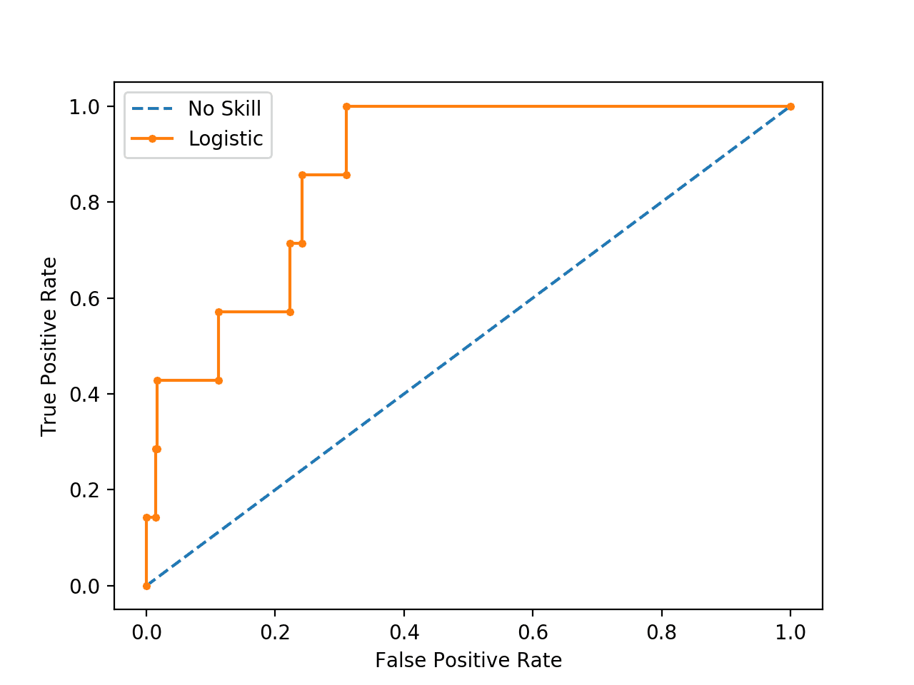
The ROC AUC scores for both classifiers are reported, showing the no skill classifier achieving the lowest score of approximately 0.5 as expected. The results for the logistic regression model suggest it has some skill with a score of about 0.869.
1
2
No Skill ROC AUC 0.490
Logistic ROC AUC 0.869
A ROC curve is also created for the model and the no skill classifier, showing not excellent performance, but definitely skillful performance as compared to the diagonal no skill.
Plot of ROC Curve for Logistic Regression on Imbalanced Classification Dataset
Next, we can perform an analysis of the same model fit and evaluated on the same data using the precision-recall curve and AUC score.
The complete example is listed below.
1
2
3
4
5
6
7
8
9
10
11
12
13
14
15
16
17
18
19
20
21
22
23
24
25
26
27
28
29
30
31
32
33
34
35
36
37
38
39
40
41
42
43
44
45
46
47
48
49
50
# pr curve and pr auc on an imbalanced dataset
from sklearn.datasets import make_classification
from sklearn.dummy import DummyClassifier
from sklearn.linear_model import LogisticRegression
from sklearn.model_selection import train_test_split
from sklearn.metrics import precision_recall_curve
from sklearn.metrics import auc
from matplotlib import pyplot
# plot no skill and model precision-recall curves
def plot_pr_curve(test_y,model_probs):
# calculate the no skill line as the proportion of the positive class
As before, running the example creates the imbalanced binary classification dataset.
Note: Your results may vary given the stochastic nature of the algorithm or evaluation procedure, or differences in numerical precision. Consider running the example a few times and compare the average outcome.
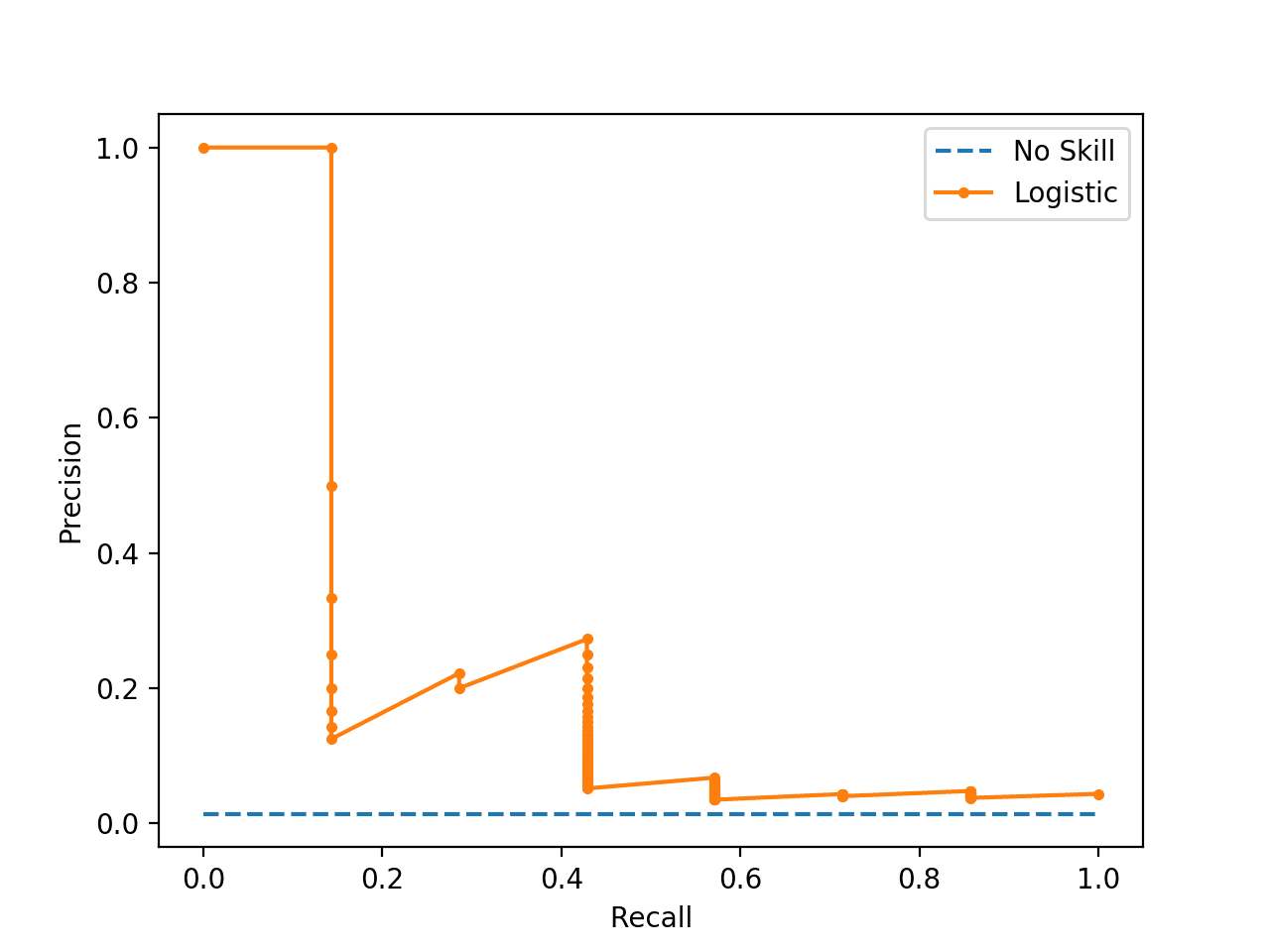
In this case we can see that the Logistic Regression model achieves a PR AUC of about 0.228 and a no skill model achieves a PR AUC of about 0.007.
1
2
No Skill PR AUC: 0.007
Logistic PR AUC: 0.228
A plot of the precision-recall curve is also created.
We can see the horizontal line of the no skill classifier as expected and in this case the zig-zag line of the logistic regression curve close to the no skill line.
Plot of Precision-Recall Curve for Logistic Regression on Imbalanced Classification Dataset
To explain why the ROC and PR curves tell a different story, recall that the PR curve focuses on the minority class, whereas the ROC curve covers both classes.
If we use a threshold of 0.5 and use the logistic regression model to make a prediction for all examples in the test set, we see that it predicts class 0 or the majority class in all cases. This can be confirmed by using the fit model to predict crisp class labels, that will use the default threshold of 0.5. The distribution of predicted class labels can then be summarized.
1
2
3
4
5
...
# predict class labels
yhat=model.predict(testX)
# summarize the distribution of class labels
print(Counter(yhat))
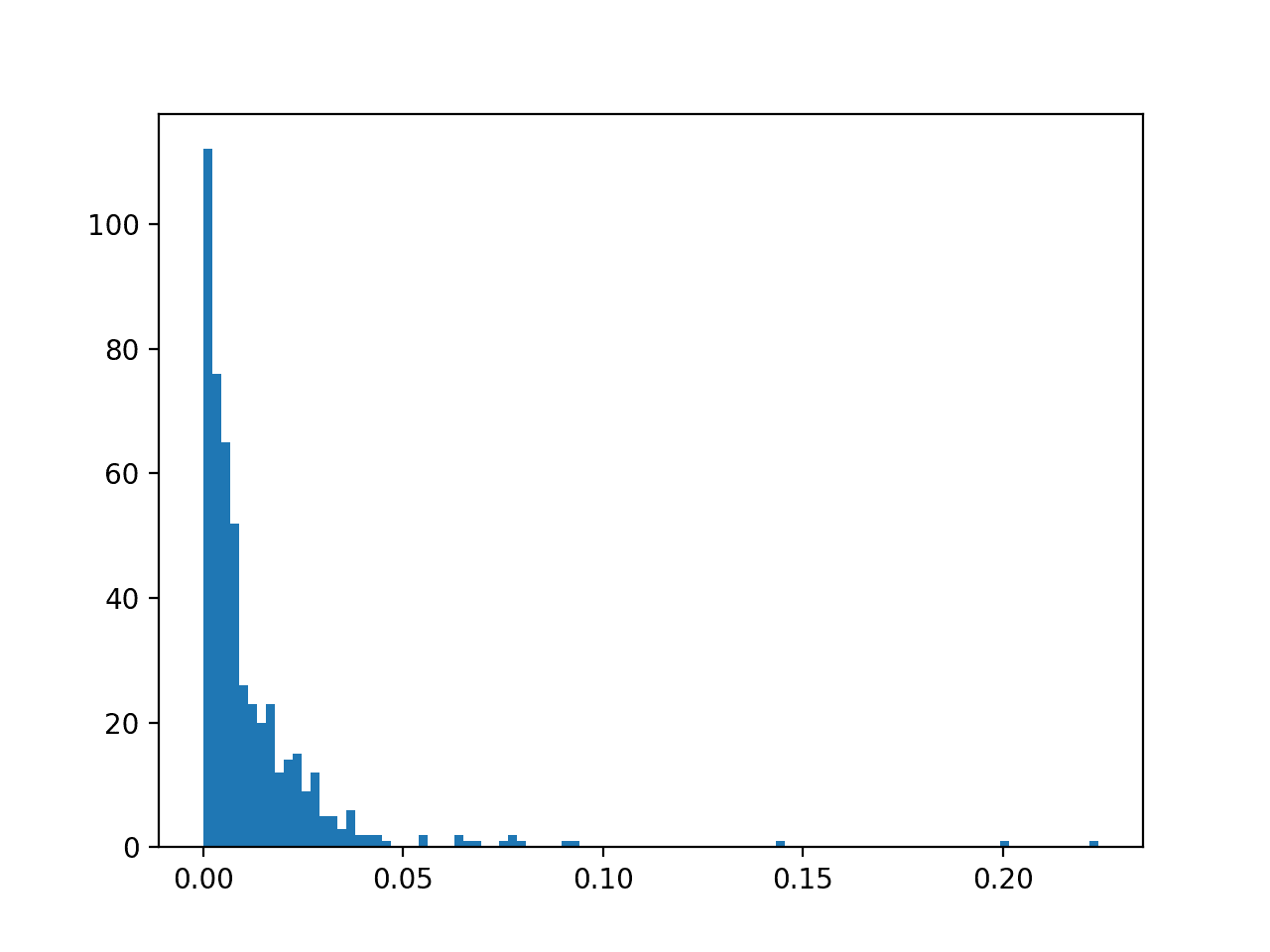
We can then create a histogram of the predicted probabilities of the positive class to confirm that the mass of predicted probabilities is below 0.5, and therefore are mapped to class 0.
1
2
3
4
...
# create a histogram of the predicted probabilities
pyplot.hist(pos_probs,bins=100)
pyplot.show()
Tying this together, the complete example is listed below.
1
2
3
4
5
6
7
8
9
10
11
12
13
14
15
16
17
18
19
20
21
22
23
24
# summarize the distribution of predicted probabilities
from collections import Counter
from matplotlib import pyplot
from sklearn.datasets import make_classification
from sklearn.linear_model import LogisticRegression
from sklearn.model_selection import train_test_split
# retrieve just the probabilities for the positive class
pos_probs=yhat[:,1]
# predict class labels
yhat=model.predict(testX)
# summarize the distribution of class labels
print(Counter(yhat))
# create a histogram of the predicted probabilities
pyplot.hist(pos_probs,bins=100)
pyplot.show()
Running the example first summarizes the distribution of predicted class labels. As we expected, the majority class (class 0) is predicted for all examples in the test set.
1
Counter({0: 500})
A histogram plot of the predicted probabilities for class 1 is also created, showing the center of mass (most predicted probabilities) is less than 0.5 and in fact is generally close to zero.
Histogram of Logistic Regression Predicted Probabilities for Class 1 for Imbalanced Classification
This means, unless probability threshold is carefully chosen, any skillful nuance in the predictions made by the model will be lost. Selecting thresholds used to interpret predicted probabilities as crisp class labels is an important topic
Further Reading
This section provides more resources on the topic if you are looking to go deeper.
It provides self-study tutorials and end-to-end projects on: Performance Metrics, Undersampling Methods, SMOTE, Threshold Moving, Probability Calibration, Cost-Sensitive Algorithms
and much more...
Bring Imbalanced Classification Methods to Your Machine Learning Projects
1. Other metrics to check for model validation are the summary of the model containing the estimates. What inference can we deduct from those estimates?
2. Reason why I said this is because if it were to be a real life situation and not random number generated from the machine.
3. Then, after discovering that the fitted model has a very low precision (i.e. <0.5) is it fair to go ahead to use this model for unseen data (predictions)?
If not, what is the way forward?
Hello Jason,
a question about Feature Extraction and Feature Selection.
Can they be classified as Unsupervised Machine Learning?
Can be useful using Feature Extraction and Feature Selection with Keras?
Can you please explain in easy words what are difference between both and what they are for?
Do you have any simple example?
Thanks a lot,
Marco
Feature selection controls which inputs from the data to feed into the model. Feature extraction provides a view or projection of the raw features as input to the model. Most neural nets will perform feature extraction automatically, e.g. a CNN for image classification.
Thanks Jason.
as far I can understand it seems to me that there is sort of sequence: first Feature selection then Feature extraction. Right?
and the result in the extraction phase maybe the same of selection (the previous phase)?
i.e. the dataset in the extraction phase maybe the same of selection?
Thanks
Perhaps. It really depends on the data and the models.
For example, ensembles of decision trees perform an automatic type of feature selection. Neural nets perform an automatic type of feature extraction, etc.
With audio/txt data and standard ml algorithms, feature extraction is pretty much a required step. On text data, not at all, unless you call it feature engineering.
Many thanks for the great article which I found super useful.
I have a question. When you stated in the very last sentence of the article “This means, unless probability threshold is carefully chosen, any skillful nuance in the predictions made by the model will be lost. Selecting thresholds used to interpret predicted probabilities as crisp class labels is an important topic”, therefore in this case, a lower probability than 0.5 needs to be taken right? For example 0.2.
Does this makes sense?
Do you have suggestions on how to pick up the best threshold in this case, or is it a matter of sorting by class 1 probabilities and taking the top N items?
I’m new at machine learning. I use a neural network for semantic segmentation to classify images in two classes. Let’s call “class 0” the majority class and “class 1” the minority class, where class 1 is the positive one.
I have grey color for class 0 and green color for class 1. I would like to create a precision-recall curve based on my neural network model but I don’t understand what is the threshold in this case.
Can you explain it to me please ?
You can collect your probability predictions and expected values and pass them to the function to calculate the curve directly. Nothing special needed.
Thank you for your answer. I’m not sure to understand. In fact, I don’t have any probability predictions and don’t know how to calculate them. Currently, I only created a neural network for semantic segmentation. For training, I gave it images and corresponding labelled images (.png images with two colors for my two classes). As output of my neural network, after training and validation, I have a test which gives me a labelled image. Which function do I have to use or how do I calculate probability predictions ? Does “expected values” corresponds to “the labelled images” in my case ?
1. How do we know this column is probability for the Class 1, i.e. Positive class? Is it the convention that the second column belongs to positive class?
# retrieve just the probabilities for the positive class
pos_probs = yhat[:, 1]
2. What exactly is this probability? does it mean the likelihood of that class to happen given a set of features? So, the sum of column 0 and 1 in the probability class is 1?
3. In the histogram plot above, I understand it shows the probability distribution for Class 1, i.e. positive class. So, here there is no observation will results in Class 1 if the threshold is 0.5? Is this correct?
ROC analysis does not have any bias toward models that perform well on the majority class at the expense of the majority class—a property that is quite attractive when dealing with imbalanced data.
I slightly confused by above statement as it has mentioned “majority class at the expense of the majority class”. I think one of them should be minority:
ROC analysis does not have any bias toward models that perform well on the minority class at the expense of the majority class—a property that is quite attractive when dealing with imbalanced data.
I found the post super interesting, however, as I’m not used to using AUPRC , I’m confused about a particular point.
I don’t quite understand why the “dummy” model used in the code uses the “stratified” strategy. What I usually build as a baseline for my ML model to beat, is a dummy model that outputs trainy.mean() for the positive class probabilities and 1-trainy.mean() for the negative class. I just found out I can build the same model using the “prior” strategy for the DummyClassifier (hooray!).
Such a model has an AUROC and AUPRC of 0.5. Doesn’t this mean that the logistic regression model shown in the “ROC and Precision-Recall Curves With a Severe Imbalance” section is actually pretty useless?
I’ve always found that AUROC and AUPRC for imbalanced problems to be pretty confusing, and I’ve been trying to use proper scoring rules such as log-loss and Brier Score to get the best model, and optimizing the classification threshold only after I’ve built the best possible model.
Anyways, I’m a fan of this site, thanks for the great post.
Hi Jason,
The roc_auc_score() by default uses average=’macro’ which does not take label imbalance into account. The class weights are ignored. Is it a proper way to compute auc for a binary classifier on imbalance data?
Hi Jason, thanks for this comprehensive post! I have a question regarding your PR curve for “no skill” classifier – I see here you’re plotting the actual precision and recall for a random guess classifier, most of the charts I’ve seen before have a diagonal line, is this purely for the purpose of comparing a 0.5 AUC_PR benchmark? Thanks!
I am observing a rather strange phenomenon when I process my data with CNN-1D. I have divided my data into training, validation and un-seen categories. I am getting a very high “validation” accuracy (92%) with the data. However, when I process totally “un-seen data”, the accuracy is near 50% (which seems to me like a chance level accuracy).
My “un-seen data” confusion matrix is below. The accuracy is 53%.
[[289 191]
[143 97]]
Could you please give me some guidelines how to justify this mismatch? I don’t understand, why the CNN converges so well? How to identify the feature which makes it converge and what is lacking with “un-seen” data?
Hello,
First of all thank you for the tutorial. I am predicting flood susceptible areas with 15 conditioning factors(both categorical and continuous variables) using support vector machine algorithm. I am observing a rather strange phenomenon when I process my data Which is my accuracy on testing data is 97.45 and area under the curve is almost 100% (actually 99.7%). I felt suspicious about that. According to you what can be the reason for this ?
You may be working on a regression problem and achieve zero prediction errors.
Alternately, you may be working on a classification problem and achieve 100% accuracy.
This is unusual and there are many possible reasons for this, including:
You are evaluating model performance on the training set by accident.
Your hold out dataset (train or validation) is too small or unrepresentative.
You have introduced a bug into your code and it is doing something different from what you expect.
Your prediction problem is easy or trivial and may not require machine learning.
The most common reason is that your hold out dataset is too small or not representative of the broader problem.
This can be addressed by:
Using k-fold cross-validation to estimate model performance instead of a train/test split.
Gather more data.
Use a different split of data for train and test, such as 50/50.
Hi!
If you switch the weights, say you put weights=[0.01, 0.99] inside make_classification, making Class 1 the dominant one, you’ll end up with a PR AUC which is bigger than the ROC AUC….! But you still have an imbalanced dataset, it doesn’t matter which class is the major one, right? So I would expect the same result as before. How do you modify the code to account for that?
Hello. Many thanks for your work. I’ve learned a lot from your channel. Quick query regarding the AUC for PR curves when using imbalanced datasets. The no_skill value (i.e. the precision for the no-skill classifier) is computed as the proportion of positive samples in the entire set. Given the PR curve for the no skill classifier (a horizontal line with y value equal to proportion of positive samples), if we wanted to get the Average Precision (approximate area under curve), would it not simply be the area of a rectangle with length =1 and height = proportion of positive samples ? Why is the dummy classifier needed when we can calculate the area directly from the no-skill PR curve ?
Hello James, thank you very much for all your posts, and efforts to share your knowledge.
I have a hard time understanding: “ROC Curves and ROC AUC can be optimistic on severely imbalanced classification problems with few samples of the minority class.”
Isn’t the class with fewer samples always the minority class ?
or by the above sentence do you mean: that data from the normal case is not sufficient in the dataset ? I am also having a hard time coming up with a real example. Can you provide one ?
I am having a hard time because I tend to think of these classes as mere labels and always label the class with fewer samples as positive. Am I thinking about this the wrong way ?
We are creating a model and train on our training set and using that model we predict the probabilities of the test set. And choose a threshold that gives us best F1 score or any other metric acc. to our needs on the test data. Now that performance metric is not reliable to new data anymore since we choose a parameter(threshold) based on our test data, it may be biased. Should we use a separate cv set to choose a threshold and give the performance of the model ion the unseen test data. Or Am I missing something here?
I have a test data set with significantly more anomalies than normal data. My anomaly detection should reliably recognise anomalies. It should not give false positives as this will lead to a system failure (classify anomaly as normal). Would you then use a PR-AUC to compare the different anomaly detections?
Alternatively, I could omit many anomalies from the test dataset so that I have the same number of anomalies as normal data and then use a ROC-AUC.
Hi Mark…Choosing between PR-AUC (Precision-Recall Area Under Curve) and ROC-AUC (Receiver Operating Characteristic Area Under Curve) depends on the specific requirements of your anomaly detection task.
1. **PR-AUC:**
– PR-AUC is a suitable metric when the dataset is highly imbalanced, such as in your case where there are significantly more anomalies than normal data.
– PR-AUC focuses on the trade-off between precision (the proportion of true anomalies among the detected anomalies) and recall (the proportion of true anomalies that are detected).
– It is particularly useful when you want to avoid false positives (classifying anomalies as normal) because precision directly measures the accuracy of the positive predictions (anomalies).
2. **ROC-AUC:**
– ROC-AUC is more suitable when the dataset is balanced or when the cost of false positives and false negatives is roughly equal.
– It evaluates the trade-off between true positive rate (TPR or recall) and false positive rate (FPR).
– ROC-AUC is less informative in highly imbalanced datasets because it can give a misleading impression of the model’s performance, especially if the majority class (normal data) dominates.
Given that your priority is to avoid false positives and reliably recognize anomalies, PR-AUC would be a better choice. It provides a more informative assessment of your model’s performance in terms of precision and recall, which are directly relevant to your task requirements.
Regarding the option of omitting many anomalies from the test dataset to balance the classes and then using ROC-AUC:
– This approach artificially balances the classes but may not reflect the real-world scenario where anomalies are prevalent.
– It might not provide a realistic evaluation of your model’s performance in handling imbalanced data and detecting anomalies.
– Using PR-AUC on the original imbalanced dataset would give a more accurate representation of your model’s performance in detecting anomalies under real-world conditions.
Therefore, I would recommend using PR-AUC to compare different anomaly detection methods, considering the highly imbalanced nature of your dataset and the importance of avoiding false positives.
Hi James,
Thanks a lot for this article, I have a question, so apparently measuring only the AUC of PR curve is not enough, you have to look at it in relation to the baseline which is not the same for all cases (in roc it’s the same, 0.5 so we can compare areas)
for example looking at arc-pr of 0.8 when the positive class ration is 0.6 is not necessarily a better model than a classifier with auc-pr of 0.4 that has 0.05 positive label ratio,
i was wondering what is a best practice to interpret AUC-PR?
apart from having the ratio of positive label match in all datasets, what is a formalize way to look at the “lift from random” using AUC-PR? is it maybe:
lift from random: AUC-PR minus Area of the baseline?
or:
lift = AUC-PR/positive frequency in the data?
Would really appreciate your help here,
also, why is the baseline of AUC-PR is the positive ratio in the data and not 0.5?
This is a really good question, and it gets to the heart of why Precision–Recall curves are often misunderstood.
The first thing to understand is why PR behaves differently from ROC.
In ROC space, a random classifier always has an AUC of 0.5, no matter how imbalanced the data is. That’s because ROC uses true positive rate and false positive rate, which are both normalized by class size. Class imbalance cancels out.
Precision–Recall does not work that way. Precision depends directly on how many positives exist in the dataset:
Precision = true positives divided by all predicted positives.
If positives are rare, a random classifier will usually be wrong when it predicts positive, so precision is low. If positives are common, even random guessing will look decent. Because of this, the baseline precision of a random model is not 0.5 — it is simply the fraction of positives in the data.
That fraction is often called the prevalence. If 5 percent of your samples are positive, a random classifier will have a precision of 0.05. If 60 percent are positive, random precision is 0.6. The PR curve of a random classifier is a horizontal line at that value, and the area under it is exactly that same number. That is why the baseline AUC-PR equals the positive class ratio.
This leads directly to the problem you pointed out: raw AUC-PR values cannot be compared across datasets with different class balances.
An AUC-PR of 0.8 when 60 percent of the data is positive is much less impressive than an AUC-PR of 0.4 when only 5 percent of the data is positive. In the first case, random guessing already gives you 0.6. In the second case, random guessing only gives you 0.05.
So the question becomes: how do we measure “lift over random” in a way that is fair and comparable?
The right way to do this is to measure how much area your model gains above the random baseline, and then normalize it by how much improvement is even possible.
There are three quantities that matter:
1. The positive class fraction, which we’ll call prevalence
2. The model’s AUC-PR
3. The maximum possible AUC-PR, which is 1
A random classifier has AUC-PR equal to the prevalence. A perfect classifier has AUC-PR equal to 1. So the total “headroom” above random is:
1 minus prevalence
Your model’s improvement over random is:
AUC-PR minus prevalence
So the normalized lift is:
(AUC-PR minus prevalence) divided by (1 minus prevalence)
This gives you a score between 0 and 1 that means something intuitive:
0 means random
1 means perfect
0.5 means you achieved half of the improvement that was possible over random
This makes PR-AUC comparable across datasets with different class imbalance.
Let’s look at your example.
Case A:
Positive rate = 0.6
AUC-PR = 0.8
Baseline = 0.6
Lift over random = 0.8 minus 0.6 = 0.2
Maximum possible lift = 1 minus 0.6 = 0.4
Normalized lift = 0.2 divided by 0.4 = 0.5
Case B:
Positive rate = 0.05
AUC-PR = 0.4
Baseline = 0.05
Lift over random = 0.4 minus 0.05 = 0.35
Maximum possible lift = 1 minus 0.05 = 0.95
Normalized lift = 0.35 divided by 0.95 = about 0.37
Now you can compare them meaningfully. The first model captured about 50 percent of the possible improvement over random. The second captured about 37 percent. So in this case the first model is actually stronger, even though its raw AUC-PR looked less impressive once you account for class balance.
Finally, to answer your specific proposals:
AUC-PR minus baseline is a good first step. It measures absolute lift over random, but it does not account for how much improvement was possible.
AUC-PR divided by prevalence is not well-behaved. It explodes when prevalence is small and does not correspond to “how close to optimal” the model is.
The normalized lift formula above is the clean, principled way to interpret PR-AUC.
Once you think of PR-AUC as “area above the prevalence line,” everything about its behavior makes sense.


Thanks for sharing, it’s a good reading!
You’re welcome!
Thanks for the tutorial.
1. Other metrics to check for model validation are the summary of the model containing the estimates. What inference can we deduct from those estimates?
2. Reason why I said this is because if it were to be a real life situation and not random number generated from the machine.
3. Then, after discovering that the fitted model has a very low precision (i.e. <0.5) is it fair to go ahead to use this model for unseen data (predictions)?
If not, what is the way forward?
If a model performs better than a naive model, then it has skill.
You can decide whether you want to use it or continue to test new models to see if you can perform better.
Testing new models ends when you run out of time/resources or when the result is good enough for project stakeholders.
Great article as usual! I appreciate all you do for the community.
Thanks Greg!
Hello Jason,
a question about Feature Extraction and Feature Selection.
Can they be classified as Unsupervised Machine Learning?
Can be useful using Feature Extraction and Feature Selection with Keras?
Can you please explain in easy words what are difference between both and what they are for?
Do you have any simple example?
Thanks a lot,
Marco
Maybe. They are not really a learning algorithm.
Yes, but it depends on the type of problem.
Feature selection controls which inputs from the data to feed into the model. Feature extraction provides a view or projection of the raw features as input to the model. Most neural nets will perform feature extraction automatically, e.g. a CNN for image classification.
Thanks Jason.
as far I can understand it seems to me that there is sort of sequence: first Feature selection then Feature extraction. Right?
and the result in the extraction phase maybe the same of selection (the previous phase)?
i.e. the dataset in the extraction phase maybe the same of selection?
Thanks
Perhaps. It really depends on the data and the models.
For example, ensembles of decision trees perform an automatic type of feature selection. Neural nets perform an automatic type of feature extraction, etc.
With audio/txt data and standard ml algorithms, feature extraction is pretty much a required step. On text data, not at all, unless you call it feature engineering.
So on. It’s complicated.
Hi
What do you exactly mean with “crisp class labels”? Especially the word crisp?
Thanks
Good question.
I mean label per sample, as opposed to probability of class membership for each sample.
Hi,
Please, it will be great if you can show us how to optimize the best threshold (lower than 0.5) for minimize False negative and False positive.
I have a tutorial on exactly this written and will appear in my new book (available soon).
Hi,
which book is this?
Imbalanced Classification with Python which came out in Jan 2020:
https://machinelearningmastery.com/imbalanced-classification-with-python/
Do you have a special offer/discount code for your new book? Thanks
Yes, see this:
https://machinelearningmastery.com/faq/single-faq/can-i-have-a-discount
How would we interpret a case In which we get perfect accuracy but zero roc-auc, f1-score, precision and recall?
It does not make sense. You may have a bug somewhere.
Hello,
Many thanks for the great article which I found super useful.
I have a question. When you stated in the very last sentence of the article “This means, unless probability threshold is carefully chosen, any skillful nuance in the predictions made by the model will be lost. Selecting thresholds used to interpret predicted probabilities as crisp class labels is an important topic”, therefore in this case, a lower probability than 0.5 needs to be taken right? For example 0.2.
Does this makes sense?
Do you have suggestions on how to pick up the best threshold in this case, or is it a matter of sorting by class 1 probabilities and taking the top N items?
Thanks and looking forward for your reply.
Jon
Yes, see this:
https://machinelearningmastery.com/threshold-moving-for-imbalanced-classification/
Hello !
I’m new at machine learning. I use a neural network for semantic segmentation to classify images in two classes. Let’s call “class 0” the majority class and “class 1” the minority class, where class 1 is the positive one.
I have grey color for class 0 and green color for class 1. I would like to create a precision-recall curve based on my neural network model but I don’t understand what is the threshold in this case.
Can you explain it to me please ?
Thanks
You can collect your probability predictions and expected values and pass them to the function to calculate the curve directly. Nothing special needed.
Hello !
Thank you for your answer. I’m not sure to understand. In fact, I don’t have any probability predictions and don’t know how to calculate them. Currently, I only created a neural network for semantic segmentation. For training, I gave it images and corresponding labelled images (.png images with two colors for my two classes). As output of my neural network, after training and validation, I have a test which gives me a labelled image. Which function do I have to use or how do I calculate probability predictions ? Does “expected values” corresponds to “the labelled images” in my case ?
Thank you very much for your help
The predict() function returns probabilities.
Yes, expected values are the labels the model is expected to predict, 0 or 1.
Recall roc curves require a binary classification task.
While this writeup is great and the motivation accurate, PR curves are very problematic and should not be used, especially not to take the AUC. Instead, use PR-gain curves. This paper (NIPS’15) explains the problems and the solution: https://papers.nips.cc/paper/5867-precision-recall-gain-curves-pr-analysis-done-right.pdf
Thanks for sharing.
Hi Jason,
Thank you for the tutorial. Few questions:
1. How do we know this column is probability for the Class 1, i.e. Positive class? Is it the convention that the second column belongs to positive class?
# retrieve just the probabilities for the positive class
pos_probs = yhat[:, 1]
2. What exactly is this probability? does it mean the likelihood of that class to happen given a set of features? So, the sum of column 0 and 1 in the probability class is 1?
3. In the histogram plot above, I understand it shows the probability distribution for Class 1, i.e. positive class. So, here there is no observation will results in Class 1 if the threshold is 0.5? Is this correct?
Thank you
You’re welcome.
Good question, yes convention, I recommend reading about the binomial distribution:
https://machinelearningmastery.com/discrete-probability-distributions-for-machine-learning/
The model predicts the probability that the input sample belongs to class=1.
The sum of the probability and 1-probability equals one, again, see the binomial distribution:
https://machinelearningmastery.com/discrete-probability-distributions-for-machine-learning/
We can choose an appropriate threshold to interpret the probabilities, called threshold moving:
https://machinelearningmastery.com/threshold-moving-for-imbalanced-classification/
ROC analysis does not have any bias toward models that perform well on the majority class at the expense of the majority class—a property that is quite attractive when dealing with imbalanced data.
I slightly confused by above statement as it has mentioned “majority class at the expense of the majority class”. I think one of them should be minority:
ROC analysis does not have any bias toward models that perform well on the minority class at the expense of the majority class—a property that is quite attractive when dealing with imbalanced data.
Request you please elaborate on this.
Thanks, fixed.
Hi Jason. Do you have a piece on using GINI as a scoring metric and why it’s good to use?
No, great suggestion though, thanks.
Hello,
I found the post super interesting, however, as I’m not used to using AUPRC , I’m confused about a particular point.
I don’t quite understand why the “dummy” model used in the code uses the “stratified” strategy. What I usually build as a baseline for my ML model to beat, is a dummy model that outputs trainy.mean() for the positive class probabilities and 1-trainy.mean() for the negative class. I just found out I can build the same model using the “prior” strategy for the DummyClassifier (hooray!).
Such a model has an AUROC and AUPRC of 0.5. Doesn’t this mean that the logistic regression model shown in the “ROC and Precision-Recall Curves With a Severe Imbalance” section is actually pretty useless?
I’ve always found that AUROC and AUPRC for imbalanced problems to be pretty confusing, and I’ve been trying to use proper scoring rules such as log-loss and Brier Score to get the best model, and optimizing the classification threshold only after I’ve built the best possible model.
Anyways, I’m a fan of this site, thanks for the great post.
This may help with understanding the metrics:
https://machinelearningmastery.com/tour-of-evaluation-metrics-for-imbalanced-classification/
This may help for choosing a naive model for metrics:
https://machinelearningmastery.com/naive-classifiers-imbalanced-classification-metrics/
Hi Jason,
The roc_auc_score() by default uses average=’macro’ which does not take label imbalance into account. The class weights are ignored. Is it a proper way to compute auc for a binary classifier on imbalance data?
Depends on your goal – what you want to measure.
Hi. How can we use the above metrics for multiclass problem? Any reading on that?
Generally you cannot.
There are extensions that try, I’m not across them sorry. Try scholar.google.com
Hi Jason, thanks for this comprehensive post! I have a question regarding your PR curve for “no skill” classifier – I see here you’re plotting the actual precision and recall for a random guess classifier, most of the charts I’ve seen before have a diagonal line, is this purely for the purpose of comparing a 0.5 AUC_PR benchmark? Thanks!
Yes, a diagonal line is used for ROC curves, a flat line for precision-recall curves.
Hello Jason,
I am observing a rather strange phenomenon when I process my data with CNN-1D. I have divided my data into training, validation and un-seen categories. I am getting a very high “validation” accuracy (92%) with the data. However, when I process totally “un-seen data”, the accuracy is near 50% (which seems to me like a chance level accuracy).
Please refer to my “training and validation graph” in the below link.
https://drive.google.com/file/d/10pGQG0YsVNMIM7g0YEWdOmzM2lv5l3Ss/view?usp=sharing
My “un-seen data” confusion matrix is below. The accuracy is 53%.
[[289 191]
[143 97]]
Could you please give me some guidelines how to justify this mismatch? I don’t understand, why the CNN converges so well? How to identify the feature which makes it converge and what is lacking with “un-seen” data?
Regards,
Swati.
Hi Swati…One consideration would be the relative size of the datasets being used.
Hello,
First of all thank you for the tutorial. I am predicting flood susceptible areas with 15 conditioning factors(both categorical and continuous variables) using support vector machine algorithm. I am observing a rather strange phenomenon when I process my data Which is my accuracy on testing data is 97.45 and area under the curve is almost 100% (actually 99.7%). I felt suspicious about that. According to you what can be the reason for this ?
Hi Kumudu,
You may be working on a regression problem and achieve zero prediction errors.
Alternately, you may be working on a classification problem and achieve 100% accuracy.
This is unusual and there are many possible reasons for this, including:
You are evaluating model performance on the training set by accident.
Your hold out dataset (train or validation) is too small or unrepresentative.
You have introduced a bug into your code and it is doing something different from what you expect.
Your prediction problem is easy or trivial and may not require machine learning.
The most common reason is that your hold out dataset is too small or not representative of the broader problem.
This can be addressed by:
Using k-fold cross-validation to estimate model performance instead of a train/test split.
Gather more data.
Use a different split of data for train and test, such as 50/50.
Hi!
If you switch the weights, say you put weights=[0.01, 0.99] inside make_classification, making Class 1 the dominant one, you’ll end up with a PR AUC which is bigger than the ROC AUC….! But you still have an imbalanced dataset, it doesn’t matter which class is the major one, right? So I would expect the same result as before. How do you modify the code to account for that?
Thanks.
Hi GiaZ…The following resource is a great starting point to understand the fundamentals of best practices when working with imbalanced classification.
https://machinelearningmastery.com/framework-for-imbalanced-classification-projects/
Hello.
What is better in case of imbalanced data… the Matthews score (also called phi or mcc) or the Fowlkes score?
I know these are only calculated for a single threshold point.
Hello, Thank you
Which measure is important in imbalanced data?
You are very welcome Ali! The following resource provides a tour of evaluation metrics for imbalanced classification:
https://machinelearningmastery.com/tour-of-evaluation-metrics-for-imbalanced-classification/#:~:text=There%20are%20two%20groups%20of,%2Dspecificity%20and%20precision%2Drecall.
Hello. Many thanks for your work. I’ve learned a lot from your channel. Quick query regarding the AUC for PR curves when using imbalanced datasets. The no_skill value (i.e. the precision for the no-skill classifier) is computed as the proportion of positive samples in the entire set. Given the PR curve for the no skill classifier (a horizontal line with y value equal to proportion of positive samples), if we wanted to get the Average Precision (approximate area under curve), would it not simply be the area of a rectangle with length =1 and height = proportion of positive samples ? Why is the dummy classifier needed when we can calculate the area directly from the no-skill PR curve ?
Hi Suraj…You may certainly use your approach. Let us know what differences you note from both methods.
Hello James, thank you very much for all your posts, and efforts to share your knowledge.
I have a hard time understanding: “ROC Curves and ROC AUC can be optimistic on severely imbalanced classification problems with few samples of the minority class.”
Isn’t the class with fewer samples always the minority class ?
or by the above sentence do you mean: that data from the normal case is not sufficient in the dataset ? I am also having a hard time coming up with a real example. Can you provide one ?
I am having a hard time because I tend to think of these classes as mere labels and always label the class with fewer samples as positive. Am I thinking about this the wrong way ?
You are very welcome Samy! The following resource may be of interest to you:
https://machinelearningmastery.com/imbalanced-classification-is-hard/
We are creating a model and train on our training set and using that model we predict the probabilities of the test set. And choose a threshold that gives us best F1 score or any other metric acc. to our needs on the test data. Now that performance metric is not reliable to new data anymore since we choose a parameter(threshold) based on our test data, it may be biased. Should we use a separate cv set to choose a threshold and give the performance of the model ion the unseen test data. Or Am I missing something here?
Hi Karthikeyan…The following provides best practices regarding training, testing and validating and the associated datasets:
https://machinelearningmastery.com/training-validation-test-split-and-cross-validation-done-right/
I have a test data set with significantly more anomalies than normal data. My anomaly detection should reliably recognise anomalies. It should not give false positives as this will lead to a system failure (classify anomaly as normal). Would you then use a PR-AUC to compare the different anomaly detections?
Alternatively, I could omit many anomalies from the test dataset so that I have the same number of anomalies as normal data and then use a ROC-AUC.
Hi Mark…Choosing between PR-AUC (Precision-Recall Area Under Curve) and ROC-AUC (Receiver Operating Characteristic Area Under Curve) depends on the specific requirements of your anomaly detection task.
1. **PR-AUC:**
– PR-AUC is a suitable metric when the dataset is highly imbalanced, such as in your case where there are significantly more anomalies than normal data.
– PR-AUC focuses on the trade-off between precision (the proportion of true anomalies among the detected anomalies) and recall (the proportion of true anomalies that are detected).
– It is particularly useful when you want to avoid false positives (classifying anomalies as normal) because precision directly measures the accuracy of the positive predictions (anomalies).
2. **ROC-AUC:**
– ROC-AUC is more suitable when the dataset is balanced or when the cost of false positives and false negatives is roughly equal.
– It evaluates the trade-off between true positive rate (TPR or recall) and false positive rate (FPR).
– ROC-AUC is less informative in highly imbalanced datasets because it can give a misleading impression of the model’s performance, especially if the majority class (normal data) dominates.
Given that your priority is to avoid false positives and reliably recognize anomalies, PR-AUC would be a better choice. It provides a more informative assessment of your model’s performance in terms of precision and recall, which are directly relevant to your task requirements.
Regarding the option of omitting many anomalies from the test dataset to balance the classes and then using ROC-AUC:
– This approach artificially balances the classes but may not reflect the real-world scenario where anomalies are prevalent.
– It might not provide a realistic evaluation of your model’s performance in handling imbalanced data and detecting anomalies.
– Using PR-AUC on the original imbalanced dataset would give a more accurate representation of your model’s performance in detecting anomalies under real-world conditions.
Therefore, I would recommend using PR-AUC to compare different anomaly detection methods, considering the highly imbalanced nature of your dataset and the importance of avoiding false positives.
Hi James,
Thanks a lot for this article, I have a question, so apparently measuring only the AUC of PR curve is not enough, you have to look at it in relation to the baseline which is not the same for all cases (in roc it’s the same, 0.5 so we can compare areas)
for example looking at arc-pr of 0.8 when the positive class ration is 0.6 is not necessarily a better model than a classifier with auc-pr of 0.4 that has 0.05 positive label ratio,
i was wondering what is a best practice to interpret AUC-PR?
apart from having the ratio of positive label match in all datasets, what is a formalize way to look at the “lift from random” using AUC-PR? is it maybe:
lift from random: AUC-PR minus Area of the baseline?
or:
lift = AUC-PR/positive frequency in the data?
Would really appreciate your help here,
also, why is the baseline of AUC-PR is the positive ratio in the data and not 0.5?
Thanks a lot,
Michal
Hi Michal…
This is a really good question, and it gets to the heart of why Precision–Recall curves are often misunderstood.
The first thing to understand is why PR behaves differently from ROC.
In ROC space, a random classifier always has an AUC of 0.5, no matter how imbalanced the data is. That’s because ROC uses true positive rate and false positive rate, which are both normalized by class size. Class imbalance cancels out.
Precision–Recall does not work that way. Precision depends directly on how many positives exist in the dataset:
Precision = true positives divided by all predicted positives.
If positives are rare, a random classifier will usually be wrong when it predicts positive, so precision is low. If positives are common, even random guessing will look decent. Because of this, the baseline precision of a random model is not 0.5 — it is simply the fraction of positives in the data.
That fraction is often called the prevalence. If 5 percent of your samples are positive, a random classifier will have a precision of 0.05. If 60 percent are positive, random precision is 0.6. The PR curve of a random classifier is a horizontal line at that value, and the area under it is exactly that same number. That is why the baseline AUC-PR equals the positive class ratio.
This leads directly to the problem you pointed out: raw AUC-PR values cannot be compared across datasets with different class balances.
An AUC-PR of 0.8 when 60 percent of the data is positive is much less impressive than an AUC-PR of 0.4 when only 5 percent of the data is positive. In the first case, random guessing already gives you 0.6. In the second case, random guessing only gives you 0.05.
So the question becomes: how do we measure “lift over random” in a way that is fair and comparable?
The right way to do this is to measure how much area your model gains above the random baseline, and then normalize it by how much improvement is even possible.
There are three quantities that matter:
1. The positive class fraction, which we’ll call prevalence
2. The model’s AUC-PR
3. The maximum possible AUC-PR, which is 1
A random classifier has AUC-PR equal to the prevalence. A perfect classifier has AUC-PR equal to 1. So the total “headroom” above random is:
1 minus prevalence
Your model’s improvement over random is:
AUC-PR minus prevalence
So the normalized lift is:
(AUC-PR minus prevalence) divided by (1 minus prevalence)
This gives you a score between 0 and 1 that means something intuitive:
0 means random
1 means perfect
0.5 means you achieved half of the improvement that was possible over random
This makes PR-AUC comparable across datasets with different class imbalance.
Let’s look at your example.
Case A:
Positive rate = 0.6
AUC-PR = 0.8
Baseline = 0.6
Lift over random = 0.8 minus 0.6 = 0.2
Maximum possible lift = 1 minus 0.6 = 0.4
Normalized lift = 0.2 divided by 0.4 = 0.5
Case B:
Positive rate = 0.05
AUC-PR = 0.4
Baseline = 0.05
Lift over random = 0.4 minus 0.05 = 0.35
Maximum possible lift = 1 minus 0.05 = 0.95
Normalized lift = 0.35 divided by 0.95 = about 0.37
Now you can compare them meaningfully. The first model captured about 50 percent of the possible improvement over random. The second captured about 37 percent. So in this case the first model is actually stronger, even though its raw AUC-PR looked less impressive once you account for class balance.
Finally, to answer your specific proposals:
AUC-PR minus baseline is a good first step. It measures absolute lift over random, but it does not account for how much improvement was possible.
AUC-PR divided by prevalence is not well-behaved. It explodes when prevalence is small and does not correspond to “how close to optimal” the model is.
The normalized lift formula above is the clean, principled way to interpret PR-AUC.
Once you think of PR-AUC as “area above the prevalence line,” everything about its behavior makes sense.