How to Use Polynomial Feature Transforms for Machine Learning

By Jason Brownlee on August 28, 2020 in Data Preparation 42

Often, the input features for a predictive modeling task interact in unexpected and often nonlinear ways.

These interactions can be identified and modeled by a learning algorithm. Another approach is to engineer new features that expose these interactions and see if they improve model performance. Additionally, transforms like raising input variables to a power can help to better expose the important relationships between input variables and the target variable.

These features are called interaction and polynomial features and allow the use of simpler modeling algorithms as some of the complexity of interpreting the input variables and their relationships is pushed back to the data preparation stage. Sometimes these features can result in improved modeling performance, although at the cost of adding thousands or even millions of additional input variables.

In this tutorial, you will discover how to use polynomial feature transforms for feature engineering with numerical input variables.

After completing this tutorial, you will know:

Some machine learning algorithms prefer or perform better with polynomial input features.
How to use the polynomial features transform to create new versions of input variables for predictive modeling.
How the degree of the polynomial impacts the number of input features created by the transform.

Kick-start your project with my new book Data Preparation for Machine Learning, including step-by-step tutorials and the Python source code files for all examples.

Let’s get started.

How to Use Polynomial Features Transforms for Machine Learning

How to Use Polynomial Feature Transforms for Machine Learning
Photo by D Coetzee, some rights reserved.

Tutorial Overview

This tutorial is divided into five parts; they are:

Polynomial Features
Polynomial Feature Transform
Sonar Dataset
Polynomial Feature Transform Example
Effect of Polynomial Degree

Polynomial Features

Polynomial features are those features created by raising existing features to an exponent.

For example, if a dataset had one input feature X, then a polynomial feature would be the addition of a new feature (column) where values were calculated by squaring the values in X, e.g. X^2. This process can be repeated for each input variable in the dataset, creating a transformed version of each.

As such, polynomial features are a type of feature engineering, e.g. the creation of new input features based on the existing features.

The “degree” of the polynomial is used to control the number of features added, e.g. a degree of 3 will add two new variables for each input variable. Typically a small degree is used such as 2 or 3.

Generally speaking, it is unusual to use d greater than 3 or 4 because for large values of d, the polynomial curve can become overly flexible and can take on some very strange shapes.

— Page 266, An Introduction to Statistical Learning with Applications in R, 2014.

It is also common to add new variables that represent the interaction between features, e.g a new column that represents one variable multiplied by another. This too can be repeated for each input variable creating a new “interaction” variable for each pair of input variables.

A squared or cubed version of an input variable will change the probability distribution, separating the small and large values, a separation that is increased with the size of the exponent.

This separation can help some machine learning algorithms make better predictions and is common for regression predictive modeling tasks and generally tasks that have numerical input variables.

Typically linear algorithms, such as linear regression and logistic regression, respond well to the use of polynomial input variables.

Linear regression is linear in the model parameters and adding polynomial terms to the model can be an effective way of allowing the model to identify nonlinear patterns.

— Page 11, Feature Engineering and Selection, 2019.

For example, when used as input to a linear regression algorithm, the method is more broadly referred to as polynomial regression.

Polynomial regression extends the linear model by adding extra predictors, obtained by raising each of the original predictors to a power. For example, a cubic regression uses three variables, X, X2, and X3, as predictors. This approach provides a simple way to provide a non-linear fit to data.

— Page 265, An Introduction to Statistical Learning with Applications in R, 2014.

Want to Get Started With Data Preparation?

Take my free 7-day email crash course now (with sample code).

Click to sign-up and also get a free PDF Ebook version of the course.

Polynomial Feature Transform

The polynomial features transform is available in the scikit-learn Python machine learning library via the PolynomialFeatures class.

The features created include:

The bias (the value of 1.0)
Values raised to a power for each degree (e.g. x^1, x^2, x^3, …)
Interactions between all pairs of features (e.g. x1 * x2, x1 * x3, …)

For example, with two input variables with values 2 and 3 and a degree of 2, the features created would be:

1 (the bias)
2^1 = 2
3^1 = 3
2^2 = 4
3^2 = 9
2 * 3 = 6

We can demonstrate this with an example:

# demonstrate the types of features created
from numpy import asarray
from sklearn.preprocessing import PolynomialFeatures
# define the dataset
data = asarray([[2,3],[2,3],[2,3]])
print(data)
# perform a polynomial features transform of the dataset
trans = PolynomialFeatures(degree=2)
data = trans.fit_transform(data)
print(data)

# demonstrate the types of features created

from numpy import asarray

from sklearn.preprocessing import PolynomialFeatures

# define the dataset

data = asarray([[2,3],[2,3],[2,3]])

print(data)

# perform a polynomial features transform of the dataset

trans = PolynomialFeatures(degree=2)

data = trans.fit_transform(data)

print(data)

Running the example first reports the raw data with two features (columns) and each feature has the same value, either 2 or 3.

Then the polynomial features are created, resulting in six features, matching what was described above.

[[2 3]
 [2 3]
 [2 3]]

[[1. 2. 3. 4. 6. 9.]
 [1. 2. 3. 4. 6. 9.]
 [1. 2. 3. 4. 6. 9.]]

[[2 3]

[2 3]

[2 3]]

[[1. 2. 3. 4. 6. 9.]

[1. 2. 3. 4. 6. 9.]

[1. 2. 3. 4. 6. 9.]]

The “degree” argument controls the number of features created and defaults to 2.

The “interaction_only” argument means that only the raw values (degree 1) and the interaction (pairs of values multiplied with each other) are included, defaulting to False.

The “include_bias” argument defaults to True to include the bias feature.

We will take a closer look at how to use the polynomial feature transforms on a real dataset.

First, let’s introduce a real dataset.

Sonar Dataset

The sonar dataset is a standard machine learning dataset for binary classification.

It involves 60 real-valued inputs and a two-class target variable. There are 208 examples in the dataset and the classes are reasonably balanced.

A baseline classification algorithm can achieve a classification accuracy of about 53.4 percent using repeated stratified 10-fold cross-validation. Top performance on this dataset is about 88 percent using repeated stratified 10-fold cross-validation.

The dataset describes radar returns of rocks or simulated mines.

You can learn more about the dataset from here:

No need to download the dataset; we will download it automatically from our worked examples.

First, let’s load and summarize the dataset. The complete example is listed below.

# load and summarize the sonar dataset
from pandas import read_csv
from pandas.plotting import scatter_matrix
from matplotlib import pyplot
# Load dataset
url = "https://raw.githubusercontent.com/jbrownlee/Datasets/master/sonar.csv"
dataset = read_csv(url, header=None)
# summarize the shape of the dataset
print(dataset.shape)
# summarize each variable
print(dataset.describe())
# histograms of the variables
dataset.hist()
pyplot.show()

# load and summarize the sonar dataset

from pandas import read_csv

from pandas.plotting import scatter_matrix

from matplotlib import pyplot

# Load dataset

url = "https://raw.githubusercontent.com/jbrownlee/Datasets/master/sonar.csv"

dataset = read_csv(url, header=None)

# summarize the shape of the dataset

print(dataset.shape)

# summarize each variable

print(dataset.describe())

# histograms of the variables

dataset.hist()

pyplot.show()

Running the example first summarizes the shape of the loaded dataset.

This confirms the 60 input variables, one output variable, and 208 rows of data.

A statistical summary of the input variables is provided showing that values are numeric and range approximately from 0 to 1.

(208, 61)
               0           1           2   ...          57          58          59
count  208.000000  208.000000  208.000000  ...  208.000000  208.000000  208.000000
mean     0.029164    0.038437    0.043832  ...    0.007949    0.007941    0.006507
std      0.022991    0.032960    0.038428  ...    0.006470    0.006181    0.005031
min      0.001500    0.000600    0.001500  ...    0.000300    0.000100    0.000600
25%      0.013350    0.016450    0.018950  ...    0.003600    0.003675    0.003100
50%      0.022800    0.030800    0.034300  ...    0.005800    0.006400    0.005300
75%      0.035550    0.047950    0.057950  ...    0.010350    0.010325    0.008525
max      0.137100    0.233900    0.305900  ...    0.044000    0.036400    0.043900

[8 rows x 60 columns]

(208, 61)

0 1 2 ... 57 58 59

count 208.000000 208.000000 208.000000 ... 208.000000 208.000000 208.000000

mean 0.029164 0.038437 0.043832 ... 0.007949 0.007941 0.006507

std 0.022991 0.032960 0.038428 ... 0.006470 0.006181 0.005031

min 0.001500 0.000600 0.001500 ... 0.000300 0.000100 0.000600

25% 0.013350 0.016450 0.018950 ... 0.003600 0.003675 0.003100

50% 0.022800 0.030800 0.034300 ... 0.005800 0.006400 0.005300

75% 0.035550 0.047950 0.057950 ... 0.010350 0.010325 0.008525

max 0.137100 0.233900 0.305900 ... 0.044000 0.036400 0.043900

[8 rows x 60 columns]

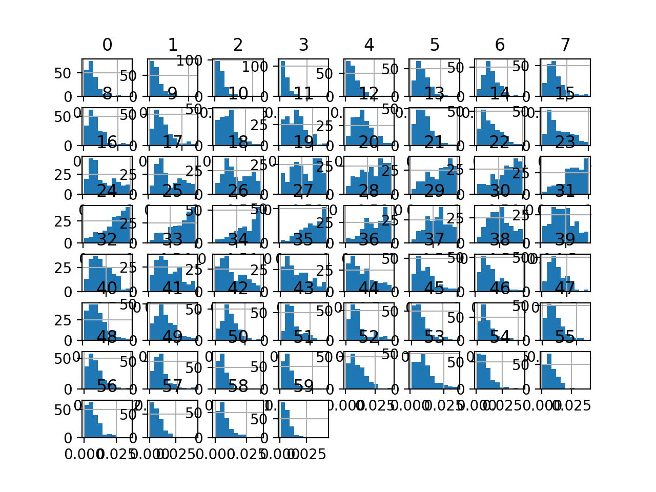
Finally, a histogram is created for each input variable.

If we ignore the clutter of the plots and focus on the histograms themselves, we can see that many variables have a skewed distribution.

Histogram Plots of Input Variables for the Sonar Binary Classification Dataset

Next, let’s fit and evaluate a machine learning model on the raw dataset.

We will use a k-nearest neighbor algorithm with default hyperparameters and evaluate it using repeated stratified k-fold cross-validation. The complete example is listed below.

# evaluate knn on the raw sonar dataset
from numpy import mean
from numpy import std
from pandas import read_csv
from sklearn.model_selection import cross_val_score
from sklearn.model_selection import RepeatedStratifiedKFold
from sklearn.neighbors import KNeighborsClassifier
from sklearn.preprocessing import LabelEncoder
from matplotlib import pyplot
# load dataset
url = "https://raw.githubusercontent.com/jbrownlee/Datasets/master/sonar.csv"
dataset = read_csv(url, header=None)
data = dataset.values
# separate into input and output columns
X, y = data[:, :-1], data[:, -1]
# ensure inputs are floats and output is an integer label
X = X.astype('float32')
y = LabelEncoder().fit_transform(y.astype('str'))
# define and configure the model
model = KNeighborsClassifier()
# evaluate the model
cv = RepeatedStratifiedKFold(n_splits=10, n_repeats=3, random_state=1)
n_scores = cross_val_score(model, X, y, scoring='accuracy', cv=cv, n_jobs=-1, error_score='raise')
# report model performance
print('Accuracy: %.3f (%.3f)' % (mean(n_scores), std(n_scores)))

# evaluate knn on the raw sonar dataset

from numpy import mean

from numpy import std

from pandas import read_csv

from sklearn.model_selection import cross_val_score

from sklearn.model_selection import RepeatedStratifiedKFold

from sklearn.neighbors import KNeighborsClassifier

from sklearn.preprocessing import LabelEncoder

from matplotlib import pyplot

# load dataset

url = "https://raw.githubusercontent.com/jbrownlee/Datasets/master/sonar.csv"

dataset = read_csv(url, header=None)

data = dataset.values

# separate into input and output columns

X, y = data[:, :-1], data[:, -1]

# ensure inputs are floats and output is an integer label

X = X.astype('float32')

y = LabelEncoder().fit_transform(y.astype('str'))

# define and configure the model

model = KNeighborsClassifier()

# evaluate the model

cv = RepeatedStratifiedKFold(n_splits=10, n_repeats=3, random_state=1)

n_scores = cross_val_score(model, X, y, scoring='accuracy', cv=cv, n_jobs=-1, error_score='raise')

# report model performance

print('Accuracy: %.3f (%.3f)' % (mean(n_scores), std(n_scores)))

Running the example evaluates a KNN model on the raw sonar dataset.

Note: Your results may vary given the stochastic nature of the algorithm or evaluation procedure, or differences in numerical precision. Consider running the example a few times and compare the average outcome.

We can see that the model achieved a mean classification accuracy of about 79.7 percent, showing that it has skill (better than 53.4 percent) and is in the ball-park of good performance (88 percent).

Accuracy: 0.797 (0.073)

1	Accuracy: 0.797 (0.073)

Next, let’s explore a polynomial features transform of the dataset.

Polynomial Feature Transform Example

We can apply the polynomial features transform to the Sonar dataset directly.

In this case, we will use a degree of 3.

...
# perform a polynomial features transform of the dataset
trans = PolynomialFeatures(degree=3)
data = trans.fit_transform(data)

...

# perform a polynomial features transform of the dataset

trans = PolynomialFeatures(degree=3)

data = trans.fit_transform(data)

Let’s try it on our sonar dataset.

The complete example of creating a polynomial features transform of the sonar dataset and summarizing the created features is below.

# visualize a polynomial features transform of the sonar dataset
from pandas import read_csv
from pandas import DataFrame
from pandas.plotting import scatter_matrix
from sklearn.preprocessing import PolynomialFeatures
from matplotlib import pyplot
# load dataset
url = "https://raw.githubusercontent.com/jbrownlee/Datasets/master/sonar.csv"
dataset = read_csv(url, header=None)
# retrieve just the numeric input values
data = dataset.values[:, :-1]
# perform a polynomial features transform of the dataset
trans = PolynomialFeatures(degree=3)
data = trans.fit_transform(data)
# convert the array back to a dataframe
dataset = DataFrame(data)
# summarize
print(dataset.shape)

# visualize a polynomial features transform of the sonar dataset

from pandas import read_csv

from pandas import DataFrame

from pandas.plotting import scatter_matrix

from sklearn.preprocessing import PolynomialFeatures

from matplotlib import pyplot

# load dataset

url = "https://raw.githubusercontent.com/jbrownlee/Datasets/master/sonar.csv"

dataset = read_csv(url, header=None)

# retrieve just the numeric input values

data = dataset.values[:, :-1]

# perform a polynomial features transform of the dataset

trans = PolynomialFeatures(degree=3)

data = trans.fit_transform(data)

# convert the array back to a dataframe

dataset = DataFrame(data)

# summarize

print(dataset.shape)

Running the example performs the polynomial features transform on the sonar dataset.

We can see that our features increased from 61 (60 input features) for the raw dataset to 39,711 features (39,710 input features).

(208, 39711)

1	(208, 39711)

Next, let’s evaluate the same KNN model as the previous section, but in this case on a polynomial features transform of the dataset.

The complete example is listed below.

# evaluate knn on the sonar dataset with polynomial features transform
from numpy import mean
from numpy import std
from pandas import read_csv
from sklearn.model_selection import cross_val_score
from sklearn.model_selection import RepeatedStratifiedKFold
from sklearn.neighbors import KNeighborsClassifier
from sklearn.preprocessing import LabelEncoder
from sklearn.preprocessing import PolynomialFeatures
from sklearn.pipeline import Pipeline
from matplotlib import pyplot
# load dataset
url = "https://raw.githubusercontent.com/jbrownlee/Datasets/master/sonar.csv"
dataset = read_csv(url, header=None)
data = dataset.values
# separate into input and output columns
X, y = data[:, :-1], data[:, -1]
# ensure inputs are floats and output is an integer label
X = X.astype('float32')
y = LabelEncoder().fit_transform(y.astype('str'))
# define the pipeline
trans = PolynomialFeatures(degree=3)
model = KNeighborsClassifier()
pipeline = Pipeline(steps=[('t', trans), ('m', model)])
# evaluate the pipeline
cv = RepeatedStratifiedKFold(n_splits=10, n_repeats=3, random_state=1)
n_scores = cross_val_score(pipeline, X, y, scoring='accuracy', cv=cv, n_jobs=-1, error_score='raise')
# report pipeline performance
print('Accuracy: %.3f (%.3f)' % (mean(n_scores), std(n_scores)))

# evaluate knn on the sonar dataset with polynomial features transform

from numpy import mean

from numpy import std

from pandas import read_csv

from sklearn.model_selection import cross_val_score

from sklearn.model_selection import RepeatedStratifiedKFold

from sklearn.neighbors import KNeighborsClassifier

from sklearn.preprocessing import LabelEncoder

from sklearn.preprocessing import PolynomialFeatures

from sklearn.pipeline import Pipeline

from matplotlib import pyplot

# load dataset

url = "https://raw.githubusercontent.com/jbrownlee/Datasets/master/sonar.csv"

dataset = read_csv(url, header=None)

data = dataset.values

# separate into input and output columns

X, y = data[:, :-1], data[:, -1]

# ensure inputs are floats and output is an integer label

X = X.astype('float32')

y = LabelEncoder().fit_transform(y.astype('str'))

# define the pipeline

trans = PolynomialFeatures(degree=3)

model = KNeighborsClassifier()

pipeline = Pipeline(steps=[('t', trans), ('m', model)])

# evaluate the pipeline

cv = RepeatedStratifiedKFold(n_splits=10, n_repeats=3, random_state=1)

n_scores = cross_val_score(pipeline, X, y, scoring='accuracy', cv=cv, n_jobs=-1, error_score='raise')

# report pipeline performance

print('Accuracy: %.3f (%.3f)' % (mean(n_scores), std(n_scores)))

Running the example, we can see that the polynomial features transform results in a lift in performance from 79.7 percent accuracy without the transform to about 80.0 percent with the transform.

Accuracy: 0.800 (0.077)

1	Accuracy: 0.800 (0.077)

Next, let’s explore the effect of different scaling ranges.

Effect of Polynomial Degree

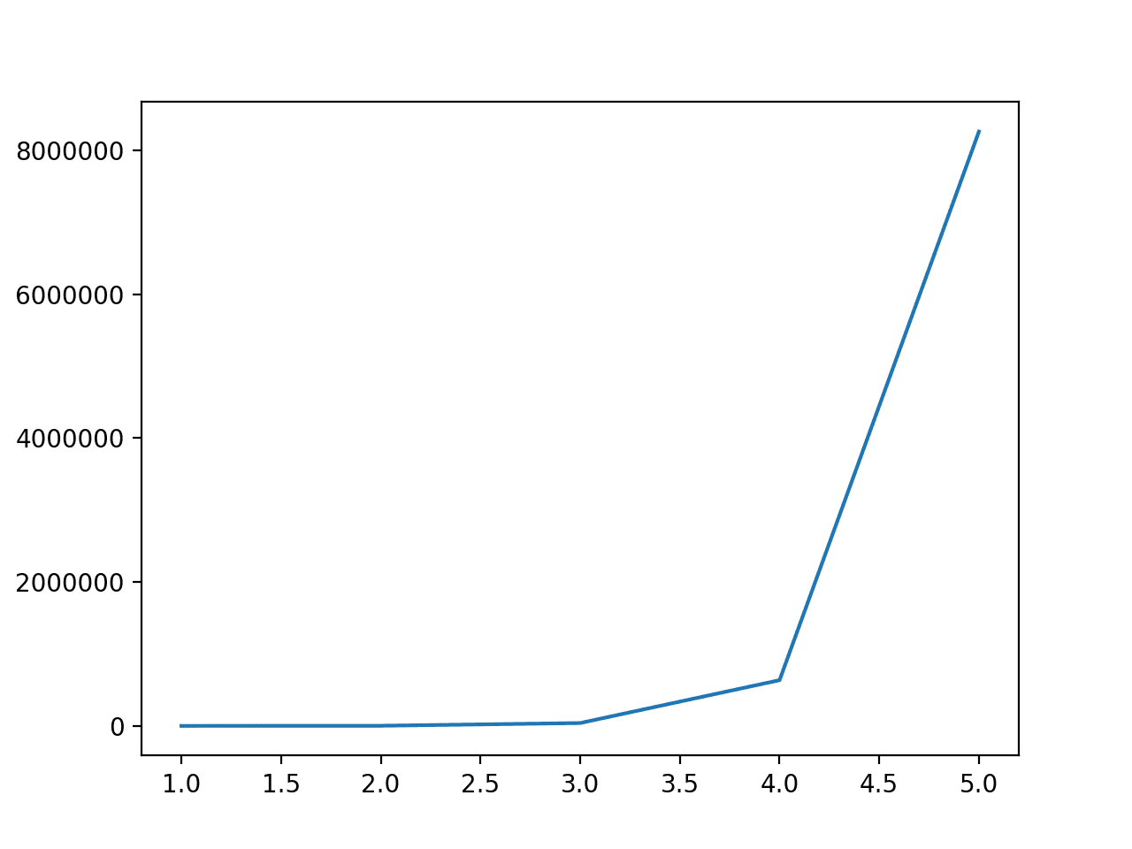
The degree of the polynomial dramatically increases the number of input features.

To get an idea of how much this impacts the number of features, we can perform the transform with a range of different degrees and compare the number of features in the dataset.

The complete example is listed below.

# compare the effect of the degree on the number of created features
from pandas import read_csv
from sklearn.preprocessing import LabelEncoder
from sklearn.preprocessing import PolynomialFeatures
from matplotlib import pyplot

# get the dataset
def get_dataset():
	# load dataset
	url = "https://raw.githubusercontent.com/jbrownlee/Datasets/master/sonar.csv"
	dataset = read_csv(url, header=None)
	data = dataset.values
	# separate into input and output columns
	X, y = data[:, :-1], data[:, -1]
	# ensure inputs are floats and output is an integer label
	X = X.astype('float32')
	y = LabelEncoder().fit_transform(y.astype('str'))
	return X, y

# define dataset
X, y = get_dataset()
# calculate change in number of features
num_features = list()
degress = [i for i in range(1, 6)]
for d in degress:
	# create transform
	trans = PolynomialFeatures(degree=d)
	# fit and transform
	data = trans.fit_transform(X)
	# record number of features
	num_features.append(data.shape[1])
	# summarize
	print('Degree: %d, Features: %d' % (d, data.shape[1]))
# plot degree vs number of features
pyplot.plot(degress, num_features)
pyplot.show()

# compare the effect of the degree on the number of created features

from pandas import read_csv

from sklearn.preprocessing import LabelEncoder

from sklearn.preprocessing import PolynomialFeatures

from matplotlib import pyplot

# get the dataset

def get_dataset():

# load dataset

url = "https://raw.githubusercontent.com/jbrownlee/Datasets/master/sonar.csv"

dataset = read_csv(url, header=None)

data = dataset.values

# separate into input and output columns

X, y = data[:, :-1], data[:, -1]

# ensure inputs are floats and output is an integer label

X = X.astype('float32')

y = LabelEncoder().fit_transform(y.astype('str'))

return X, y

# define dataset

X, y = get_dataset()

# calculate change in number of features

num_features = list()

degress = [i for i in range(1, 6)]

for d in degress:

# create transform

trans = PolynomialFeatures(degree=d)

# fit and transform

data = trans.fit_transform(X)

# record number of features

num_features.append(data.shape[1])

# summarize

print('Degree: %d, Features: %d' % (d, data.shape[1]))

# plot degree vs number of features

pyplot.plot(degress, num_features)

pyplot.show()

Running the example first reports the degree from 1 to 5 and the number of features in the dataset.

We can see that a degree of 1 has no effect and that the number of features dramatically increases from 2 through to 5.

This highlights that for anything other than very small datasets, a degree of 2 or 3 should be used to avoid a dramatic increase in input variables.

Degree: 1, Features: 61
Degree: 2, Features: 1891
Degree: 3, Features: 39711
Degree: 4, Features: 635376
Degree: 5, Features: 8259888

Degree: 1, Features: 61

Degree: 2, Features: 1891

Degree: 3, Features: 39711

Degree: 4, Features: 635376

Degree: 5, Features: 8259888

Line Plot of the Degree vs. the Number of Input Features for the Polynomial Feature Transform

More features may result in more overfitting, and in turn, worse results.

It may be a good idea to treat the degree for the polynomial features transform as a hyperparameter and test different values for your dataset.

The example below explores degree values from 1 to 4 and evaluates their effect on classification accuracy with the chosen model.

# explore the effect of degree on accuracy for the polynomial features transform
from numpy import mean
from numpy import std
from pandas import read_csv
from sklearn.model_selection import cross_val_score
from sklearn.model_selection import RepeatedStratifiedKFold
from sklearn.neighbors import KNeighborsClassifier
from sklearn.preprocessing import PolynomialFeatures
from sklearn.preprocessing import LabelEncoder
from sklearn.pipeline import Pipeline
from matplotlib import pyplot

# get the dataset
def get_dataset():
	# load dataset
	url = "https://raw.githubusercontent.com/jbrownlee/Datasets/master/sonar.csv"
	dataset = read_csv(url, header=None)
	data = dataset.values
	# separate into input and output columns
	X, y = data[:, :-1], data[:, -1]
	# ensure inputs are floats and output is an integer label
	X = X.astype('float32')
	y = LabelEncoder().fit_transform(y.astype('str'))
	return X, y

# get a list of models to evaluate
def get_models():
	models = dict()
	for d in range(1,5):
		# define the pipeline
		trans = PolynomialFeatures(degree=d)
		model = KNeighborsClassifier()
		models[str(d)] = Pipeline(steps=[('t', trans), ('m', model)])
	return models

# evaluate a give model using cross-validation
def evaluate_model(model, X, y):
	cv = RepeatedStratifiedKFold(n_splits=10, n_repeats=3, random_state=1)
	scores = cross_val_score(model, X, y, scoring='accuracy', cv=cv, n_jobs=-1, error_score='raise')
	return scores

# define dataset
X, y = get_dataset()
# get the models to evaluate
models = get_models()
# evaluate the models and store results
results, names = list(), list()
for name, model in models.items():
	scores = evaluate_model(model, X, y)
	results.append(scores)
	names.append(name)
	print('>%s %.3f (%.3f)' % (name, mean(scores), std(scores)))
# plot model performance for comparison
pyplot.boxplot(results, labels=names, showmeans=True)
pyplot.show()

# explore the effect of degree on accuracy for the polynomial features transform

from numpy import mean

from numpy import std

from pandas import read_csv

from sklearn.model_selection import cross_val_score

from sklearn.model_selection import RepeatedStratifiedKFold

from sklearn.neighbors import KNeighborsClassifier

from sklearn.preprocessing import PolynomialFeatures

from sklearn.preprocessing import LabelEncoder

from sklearn.pipeline import Pipeline

from matplotlib import pyplot

# get the dataset

def get_dataset():

# load dataset

url = "https://raw.githubusercontent.com/jbrownlee/Datasets/master/sonar.csv"

dataset = read_csv(url, header=None)

data = dataset.values

# separate into input and output columns

X, y = data[:, :-1], data[:, -1]

# ensure inputs are floats and output is an integer label

X = X.astype('float32')

y = LabelEncoder().fit_transform(y.astype('str'))

return X, y

# get a list of models to evaluate

def get_models():

models = dict()

for d in range(1,5):

# define the pipeline

trans = PolynomialFeatures(degree=d)

model = KNeighborsClassifier()

models[str(d)] = Pipeline(steps=[('t', trans), ('m', model)])

return models

# evaluate a give model using cross-validation

def evaluate_model(model, X, y):

cv = RepeatedStratifiedKFold(n_splits=10, n_repeats=3, random_state=1)

scores = cross_val_score(model, X, y, scoring='accuracy', cv=cv, n_jobs=-1, error_score='raise')

return scores

# define dataset

X, y = get_dataset()

# get the models to evaluate

models = get_models()

# evaluate the models and store results

results, names = list(), list()

for name, model in models.items():

scores = evaluate_model(model, X, y)

results.append(scores)

names.append(name)

print('>%s %.3f (%.3f)' % (name, mean(scores), std(scores)))

# plot model performance for comparison

pyplot.boxplot(results, labels=names, showmeans=True)

pyplot.show()

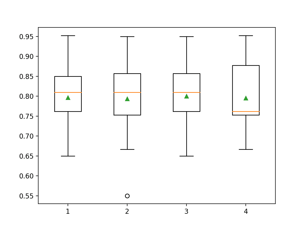
Running the example reports the mean classification accuracy for each polynomial degree.

In this case, we can see that performance is generally worse than no transform (degree 1) except for a degree 3.

It might be interesting to explore scaling the data before or after performing the transform to see how it impacts model performance.

>1 0.797 (0.073)
>2 0.793 (0.085)
>3 0.800 (0.077)
>4 0.795 (0.079)

>1 0.797 (0.073)

>2 0.793 (0.085)

>3 0.800 (0.077)

>4 0.795 (0.079)

Box and whisker plots are created to summarize the classification accuracy scores for each polynomial degree.

We can see that performance remains flat, perhaps with the first signs of overfitting with a degree of 4.

Box Plots of Degree for the Polynomial Feature Transform vs. Classification Accuracy of KNN on the Sonar Dataset

Summary

In this tutorial, you discovered how to use polynomial feature transforms for feature engineering with numerical input variables.

Specifically, you learned:

Some machine learning algorithms prefer or perform better with polynomial input features.
How to use the polynomial features transform to create new versions of input variables for predictive modeling.
How the degree of the polynomial impacts the number of input features created by the transform.

Do you have any questions?
Ask your questions in the comments below and I will do my best to answer.

42 Responses to How to Use Polynomial Feature Transforms for Machine Learning

Faisal Alsrheed May 29, 2020 at 7:12 am #

Hello, again 🙂

I am using feedforward neural network as a regression by using (5 input features/ sensors readings).

I want to try Polynomial Feature Transform for this project to create more input features

My question is:
Can I do (RobustScaler) or (StandardScaler) after doing PolynomialFeatures?

Thank you very much

Reply
- Jason Brownlee May 29, 2020 at 1:23 pm #
  
  Yes.
  
  One approach would be to apply the transforms as part of a pipeline to your dataset, then provide the data to the model.
  
  Reply
- J May 30, 2020 at 8:28 pm #
  
  This case study is not convincing regarding the benefits of polynomial models.
  
  You started with 200 datapoints and 60 variables. After adding 1000+ variables you raised model accuracy by 0.3%.
  
  1: This level of increase can be achieved by chance, i.e. just retraining the original model.
  
  2: There is no holdout set cv. Realistically you’d have 150 observations to model with and most models would overfit without feature selection.
  
  3: It demonstrates well how OO nature of python modules is cumbersome for statistical workflows. The same can be done in R using half the LOC and twice the readability.
  
  Reply
  - Jason Brownlee May 31, 2020 at 6:23 am #
    
    Yes, I could make a better case. Thanks for the feedback.
    
    Reply
marco May 29, 2020 at 9:50 pm #

Hello Jason,
Is it possible to perform polynomial regression with Keras?
Do you have any easy example?
Thanks
Marco

Reply
- Jason Brownlee May 30, 2020 at 6:02 am #
  
  Yes, you can generate the features then pass them to your keras model.
  
  No, I don’t have an example but it should be straightforward.
  
  Reply
Gamze May 30, 2020 at 1:34 am #

Thanks for your sharing,

If we want to make predictions, should we also implement the Polynomial Feature Transform for the test data?

Thanks again

Reply
- Jason Brownlee May 30, 2020 at 6:06 am #
  
  Yes, the same transform object must be used for the train and test datasets. E.g. it is fit on the training set and applied to the train and test sets.
  
  Reply
Tina June 11, 2020 at 1:12 am #

Hello Jason,

your blog posts are incredibly interesting for a practitioner like me! This time I have a question: does the polynomial feature transform not introduce multicollinearity (e.g. correlation between x and x^2), which in turn could lead to model performance degradation?

Many thanks

Reply
- Jason Brownlee June 11, 2020 at 6:00 am #
  
  Thanks.
  
  It may which could impact some linear models.
  
  Reply

Anthony The Koala August 5, 2020 at 5:11 am #

Dear Dr Jason,
I have to say that I didn’t understand the patterns produced by the transforms of PolynomialFeatures.
I did the following with interactions and polynomials and interactions only using the array [1,2,3,4]

from numpy import asarray
from sklearn.preprocessing import PolynomialFeatures
# define the dataset
data = asarray([[1,2,3,4]])
# perform a polynomial features transform of the dataset
trans = PolynomialFeatures(degree=2)
data = trans.fit_transform(data)
data
array([[ 1.,  1.,  2.,  3.,  4.,  1.,  2.,  3.,  4.,  4.,  6.,  8.,  9.,
        12., 16.]])

from numpy import asarray

from sklearn.preprocessing import PolynomialFeatures

# define the dataset

data = asarray([[1,2,3,4]])

# perform a polynomial features transform of the dataset

trans = PolynomialFeatures(degree=2)

data = trans.fit_transform(data)

data

array([[ 1., 1., 2., 3., 4., 1., 2., 3., 4., 4., 6., 8., 9.,

12., 16.]])

With the assistance of the 2nd answer of https://stackoverflow.com/questions/51906274/cannot-understand-with-sklearns-polynomialfeatures you get the following pattern.

if data = [a,b,c,d]

1	if data = [a,b,c,d]

Then fit_transform(data) produces the form

[1, a, b, c, d, a^2, ac, ad, b^2, bc, bd,c^2,cd,d^2]

1	[1, a, b, c, d, a^2, ac, ad, b^2, bc, bd,c^2,cd,d^2]

If you exclude the the squares of a^2, b^2, c^2 and d^2.

trans2 = PolynomialFeatures(interaction_only=True); # degree = 2 by default
data = trans.fit_transform(data)
trans2.fit_transform(data)
array([[ 1.,  1.,  2.,  3.,  4.,  2.,  3.,  4.,  6.,  8., 12.]])

trans2 = PolynomialFeatures(interaction_only=True); # degree = 2 by default

data = trans.fit_transform(data)

trans2.fit_transform(data)

array([[ 1., 1., 2., 3., 4., 2., 3., 4., 6., 8., 12.]])

Which is of the type:

[1,a,b,c,d,ab,ac,ad,bc,bd,cd]

1	[1,a,b,c,d,ab,ac,ad,bc,bd,cd]

What of degree 3 and 2 values, eg data = [a,b]

trans = PolynomialFeatures(degree=3)
trans.fit([a,b])
[1,a,b,a^2,ab,b^2,a^3,a^2b,ab^2,b^3]
#if [[a,b]] = [2,3] we get
[1,2,3,4,6,9,8,12,18,27]

trans = PolynomialFeatures(degree=3)

trans.fit([a,b])

[1,a,b,a^2,ab,b^2,a^3,a^2b,ab^2,b^3]

#if [[a,b]] = [2,3] we get

[1,2,3,4,6,9,8,12,18,27]

Number of transformed outputs = (n + d)!/(n! * d!) where n = number of numbers, d = degree of polynomial.

Eg number of numbers = 3, degree of polynomial = 2,
number of transformed outputs = (n + d)! / (n! * d!) = 5!/(3! * 2!) =10

Eg number of numbers = 2, degree of polynomial = 3
number of transformed outputs = 5!/(2!*3!) = 10

Thank you,
Anthony of Sydney

Jason Brownlee August 5, 2020 at 6:21 am #

Thanks for sharing your findings.

Anthony The Koala August 5, 2020 at 6:45 am #

Dear Dr Jason,
I was experimenting with the code under the subheading “Polynomial Feature Transform Example” which is also in Listing 23.10, page 310 (327 of 398) of your book.

The particular lines of interest are:

trans = PolynomialFeatures(degree=3)
model = KNeighborsClassifier()
pipeline = Pipeline(steps=[('t', trans), ('m', model)])
# evaluate the pipeline
cv = RepeatedStratifiedKFold(n_splits=10, n_repeats=3, random_state=1)
n_scores = cross_val_score(pipeline, X, y, scoring='accuracy', cv=cv, n_jobs=-1, error_score='raise')
# report pipeline performance
mean(n_scores), std(n_scores)
(0.799920634920635, 0.07675259734559173)

trans = PolynomialFeatures(degree=3)

model = KNeighborsClassifier()

pipeline = Pipeline(steps=[('t', trans), ('m', model)])

# evaluate the pipeline

cv = RepeatedStratifiedKFold(n_splits=10, n_repeats=3, random_state=1)

n_scores = cross_val_score(pipeline, X, y, scoring='accuracy', cv=cv, n_jobs=-1, error_score='raise')

# report pipeline performance

mean(n_scores), std(n_scores)

(0.799920634920635, 0.07675259734559173)

I ask the question “,,,why didn’t the author transform by

X2 = trans.fit_transform(X)

1	X2 = trans.fit_transform(X)

and feed that into the cross_val_score?

n_scores = cross_val_score(model, X2, y, scoring='accuracy', cv=cv, n_jobs=-1)

1	n_scores = cross_val_score(model, X2, y, scoring='accuracy', cv=cv, n_jobs=-1)

Note I did not use the pipeline since BUT I used the transformed polynomial features X2.

I still got the same result.

# report pipeline performance
mean(n_scores), std(n_scores)
(0.799920634920635, 0.07675259734559173)

# report pipeline performance

mean(n_scores), std(n_scores)

(0.799920634920635, 0.07675259734559173)

The question is: In the original code the pipeline seemed to have performed the PolynomialFeatures function of degree 3 without putting the transformed(X) = X2 into the cross_val_score function.

Put it another way, in the original code, how is that pipeline managed to calculate the transformed featurs without using the transformed features in the cross_val_score. Yet I got the same result.

Thank you,
Anthony of Sydney

Jason Brownlee August 5, 2020 at 1:41 pm #

The pipeline performs the transform to the input data, and the transformed data is then passed to the model.

You can learn more about how pipelines work here:
https://scikit-learn.org/stable/modules/generated/sklearn.pipeline.Pipeline.html

Reply
- Anthony The Koala August 5, 2020 at 7:18 pm #
  
  Dear Dr Jason,
  “The pipeline performs the transform to the input data, and the transformed data is then passed to the model.”
  The issue was clarified
  Thank you.
  Anthony of Sydney.
- Jason Brownlee August 6, 2020 at 6:11 am #
  
  Happy to hear that.

Bill February 6, 2021 at 9:14 pm #

Hi Jason,
Thank you for the article, it’s very informative. My question is in regards to the application of this technique. Should the conversion of features to a polynomial be used for regression problems or can they be used for classification problems as well?
Thank you,
Bill

Reply
- Jason Brownlee February 7, 2021 at 5:18 am #
  
  Polynomial features can help on regression and classification tasks, perhaps try and compare to results of the same model without polynomial features.
  
  Reply

Erika February 22, 2021 at 2:21 am #

Hi Jason,

I have a question. What is the correct order to make in the Pipeline: StandardScale and Polynomial Features or Polynomial Features and StandardScale? I’m confused about that.

Reply
- Jason Brownlee February 22, 2021 at 5:04 am #
  
  My advice would be to test to see if it makes a difference.
  
  My gut says in this case it probably does not matter.
  
  Reply
  - Erika February 22, 2021 at 6:52 am #
    
    Got it! Thank you so much! Your website is awesome!
    
    Reply
    - Jason Brownlee February 22, 2021 at 7:37 am #
      
      You’re welcome.
      
      Thanks!
      
      Reply
Sanjeet April 12, 2021 at 6:14 am #

Hi, I have only 1 independent feature which exhibit non linear relationship with the target, should I create polynomial features from that independent variable for tree based model?

Reply
- Jason Brownlee April 13, 2021 at 6:00 am #
  
  Perhaps try it and compare results to other methods.
  
  Reply
muhammad ali raza abid April 15, 2021 at 4:04 pm #

I created polynomial features upto degree 4 and they improved my linear regression model R2 score significantly (validated by Cross Validation). However my question is that the newly created polynomial features are highly correlated to the original feature from which they are generated with pearson correlation values above 0.80. Isn’t it lead to multicollinearity problem? Or is it acceptable to accept the results of the model?

Reply
- Jason Brownlee April 16, 2021 at 5:29 am #
  
  It may be.
  
  Focus on model performance. If the model performs better, then keep the new features.
  
  Reply
  - muhammad ali raza abid April 16, 2021 at 10:21 am #
    
    Dear Jason thanks a lot for your advice. I have another question please. You mentioned with a book reference that “for large values of d (degree) the polynomial curves becomes overly flexible and can take very strange shapes”. My question is for large value of d say 5, if the linear model performance is increasing plus i do not see any abnormality in the regression line, can we keep those features to build the model?
    
    Actually in my case i have 13 features, i find out the most important feature, created 5 degree polynomial features from that single most important feature, observed considerable improvement in model performance till d=5 , and it started reducing at d=6.. I hope you understand my question. thanks in advance.
    
    Reply
    - Jason Brownlee April 17, 2021 at 6:04 am #
      
      Sure, use whatever works best for your data and test harness. Ensure your test harness is robust so that you don’t trick yourself.
      
      Reply
      - muhammad ali raza abid April 19, 2021 at 11:40 am #
        
        Thanks a lot for your replies. Highly appreciate your awesome articles always.
      - Jason Brownlee April 20, 2021 at 5:52 am #
        
        Thanks.
muhammad ali raza abid April 28, 2021 at 4:59 pm #

Hi Jason, I have a question please. What if I created a polynomial feature having VIF=5.6, p-value=0.7 facilitated to improve the Adj. R2 by 2.5%. How do I can interpret such feature?
Thanks please.

Reply
- Jason Brownlee April 29, 2021 at 6:23 am #
  
  Sorry, I try to avoid interpreting results for readers.
  
  Perhaps compare results to other methods and use what works best or looks more reliable for your specific application.
  
  Reply
muhammad ali raza abid April 29, 2021 at 9:33 am #

Thanks for your quick reply. I appreciate it. Your comments are valuable for learners like me.

Reply
- Jason Brownlee April 30, 2021 at 5:59 am #
  
  You’re welcome.
  
  Reply
shyam vaswani June 15, 2021 at 3:22 pm #

Your articles are really fantastic and full of details and explanations and examples. you are the Jedi Master! 😀

Reply
- Jason Brownlee June 16, 2021 at 6:17 am #
  
  Thanks!
  
  Reply
ángel October 13, 2021 at 10:34 pm #

with 2 input variables with values 2,3,4 and a degree of 2. Which is the order output variables?

Maybe this?
1 (the bias)
2^1
3^1
4^1
2^2
3^2
4^2
2*3
3*4

Reply
- Adrian Tam October 14, 2021 at 3:21 am #
  
  Try to replace
  data = asarray([[2,3,4],[2,3,4]])
  and you will see it is:
  1, 2^1, 3^1, 4^1, 2^2, 2*3, 2*4, 3^2, 3*4, 4^2
  
  Reply
  - ángel October 15, 2021 at 10:09 pm #
    
    but Jason Brownlee wrote above:
    “For example, with two input variables with values 2 and 3 and a degree of 2, the features created would be:
    1 (the bias)
    2^1 = 2
    3^1 = 3
    2^2 = 4
    3^2 = 9
    2 * 3 = 6”
    
    So, it seems the interactions are the last.
    
    Reply
    - Adrian Tam October 20, 2021 at 8:20 am #
      
      You look at the output of the code, not the bullet points, you will see it was in the order [2,3,4,6,9] instead.
      
      Reply
Salaf January 12, 2022 at 12:32 am #

I have generated new features through polynomial degree =2, now should I replace/discard original features or should keep all features and their poly features for regression

Reply
- James Carmichael January 12, 2022 at 10:52 am #
  
  Hi Salaf…The following may be of interest to you for understanding transformations of datasets in general:
  
  https://machinelearningmastery.com/how-to-improve-neural-network-stability-and-modeling-performance-with-data-scaling/
  
  Reply

Navigation

How to Use Polynomial Feature Transforms for Machine Learning

Tutorial Overview

Polynomial Features

Want to Get Started With Data Preparation?

Polynomial Feature Transform

Sonar Dataset

Polynomial Feature Transform Example

Effect of Polynomial Degree

Further Reading

Books

APIs

Articles

Summary

Get a Handle on Modern Data Preparation!

Prepare Your Machine Learning Data in Minutes

Bring Modern Data Preparation Techniques to
Your Machine Learning Projects

More On This Topic

42 Responses to How to Use Polynomial Feature Transforms for Machine Learning

Leave a Reply Click here to cancel reply.

Navigation

Tutorial Overview

Polynomial Features

Want to Get Started With Data Preparation?

Polynomial Feature Transform

Sonar Dataset

Polynomial Feature Transform Example

Effect of Polynomial Degree

Further Reading

Books

APIs

Articles

Summary

Get a Handle on Modern Data Preparation!

Prepare Your Machine Learning Data in Minutes

Bring Modern Data Preparation Techniques to Your Machine Learning Projects

More On This Topic

42 Responses to How to Use Polynomial Feature Transforms for Machine Learning

Leave a Reply Click here to cancel reply.

Bring Modern Data Preparation Techniques to
Your Machine Learning Projects