Monte Carlo methods are a class of techniques for randomly sampling a probability distribution.
There are many problem domains where describing or estimating the probability distribution is relatively straightforward, but calculating a desired quantity is intractable. This may be due to many reasons, such as the stochastic nature of the domain or an exponential number of random variables.
Instead, a desired quantity can be approximated by using random sampling, referred to as Monte Carlo methods. These methods were initially used around the time that the first computers were created and remain pervasive through all fields of science and engineering, including artificial intelligence and machine learning.
In this post, you will discover Monte Carlo methods for sampling probability distributions.
After reading this post, you will know:
Often, we cannot calculate a desired quantity in probability, but we can define the probability distributions for the random variables directly or indirectly.
Monte Carlo sampling a class of methods for randomly sampling from a probability distribution.
Monte Carlo sampling provides the foundation for many machine learning methods such as resampling, hyperparameter tuning, and ensemble learning.
Kick-start your project with my new book Probability for Machine Learning, including step-by-step tutorials and the Python source code files for all examples.
Let’s get started.
A Gentle Introduction to the Monte Carlo Sampling for Probability Photo by Med Cruise Guide, some rights reserved.
Overview
This tutorial is divided into three parts; they are:
Need for Sampling
What Are Monte Carlo Methods?
Examples of Monte Carlo Methods
Need for Sampling
There are many problems in probability, and more broadly in machine learning, where we cannot calculate an analytical solution directly.
In fact, there may be an argument that exact inference may be intractable for most practical probabilistic models.
For most probabilistic models of practical interest, exact inference is intractable, and so we have to resort to some form of approximation.
The desired calculation is typically a sum of a discrete distribution or integral of a continuous distribution and is intractable to calculate. The calculation may be intractable for many reasons, such as the large number of random variables, the stochastic nature of the domain, noise in the observations, the lack of observations, and more.
In problems of this kind, it is often possible to define or estimate the probability distributions for the random variables involved, either directly or indirectly via a computational simulation.
Instead of calculating the quantity directly, sampling can be used.
Sampling provides a flexible way to approximate many sums and integrals at reduced cost.
Samples can be drawn randomly from the probability distribution and used to approximate the desired quantity.
This general class of techniques for random sampling from a probability distribution is referred to as Monte Carlo methods.
Want to Learn Probability for Machine Learning
Take my free 7-day email crash course now (with sample code).
Click to sign-up and also get a free PDF Ebook version of the course.
What Are Monte Carlo Methods?
Monte Carlo methods, or MC for short, are a class of techniques for randomly sampling a probability distribution.
There are three main reasons to use Monte Carlo methods to randomly sample a probability distribution; they are:
Estimate density, gather samples to approximate the distribution of a target function.
Approximate a quantity, such as the mean or variance of a distribution.
Optimize a function, locate a sample that maximizes or minimizes the target function.
Monte Carlo methods are named for the casino in Monaco and were first developed to solve problems in particle physics at around the time of the development of the first computers and the Manhattan project for developing the first atomic bomb.
This is called a Monte Carlo approximation, named after a city in Europe known for its plush gambling casinos. Monte Carlo techniques were first developed in the area of statistical physics – in particular, during development of the atomic bomb – but are now widely used in statistics and machine learning as well.
Drawing a sample may be as simple as calculating the probability for a randomly selected event, or may be as complex as running a computational simulation, with the latter often referred to as a Monte Carlo simulation.
Multiple samples are collected and used to approximate the desired quantity.
Given the law of large numbers from statistics, the more random trials that are performed, the more accurate the approximated quantity will become.
… the law of large numbers states that if the samples x(i) are i.i.d., then the average converges almost surely to the expected value
As such, the number of samples provides control over the precision of the quantity that is being approximated, often limited by the computational complexity of drawing a sample.
By generating enough samples, we can achieve any desired level of accuracy we like. The main issue is: how do we efficiently generate samples from a probability distribution, particularly in high dimensions?
Additionally, given the central limit theorem, the distribution of the samples will form a Normal distribution, the mean of which can be taken as the approximated quantity and the variance used to provide a confidence interval for the quantity.
The central limit theorem tells us that the distribution of the average […], converges to a normal distribution […] This allows us to estimate confidence intervals around the estimate […], using the cumulative distribution of the normal density.
Direct Sampling. Sampling the distribution directly without prior information.
Importance Sampling. Sampling from a simpler approximation of the target distribution.
Rejection Sampling. Sampling from a broader distribution and only considering samples within a region of the sampled distribution.
It’s a huge topic with many books dedicated to it. Next, let’s make the idea of Monte Carlo sampling concrete with some familiar examples.
Examples of Monte Carlo Sampling
We use Monte Carlo methods all the time without thinking about it.
For example, when we define a Bernoulli distribution for a coin flip and simulate flipping a coin by sampling from this distribution, we are performing a Monte Carlo simulation. Additionally, when we sample from a uniform distribution for the integers {1,2,3,4,5,6} to simulate the roll of a dice, we are performing a Monte Carlo simulation.
We are also using the Monte Carlo method when we gather a random sample of data from the domain and estimate the probability distribution of the data using a histogram or density estimation method.
There are many examples of the use of Monte Carlo methods across a range of scientific disciplines.
For example, Monte Carlo methods can be used for:
Calculating the probability of a move by an opponent in a complex game.
Calculating the probability of a weather event in the future.
Calculating the probability of a vehicle crash under specific conditions.
The methods are used to address difficult inference in problems in applied probability, such as sampling from probabilistic graphical models.
Related is the idea of sequential Monte Carlo methods used in Bayesian models that are often referred to as particle filters.
Particle filtering (PF) is a Monte Carlo, or simulation based, algorithm for recursive Bayesian inference.
Monte Carlo methods are also pervasive in artificial intelligence and machine learning.
Many important technologies used to accomplish machine learning goals are based on drawing samples from some probability distribution and using these samples to form a Monte Carlo estimate of some desired quantity.
They provide the basis for estimating the likelihood of outcomes in artificial intelligence problems via simulation, such as robotics. More simply, Monte Carlo methods are used to solve intractable integration problems, such as firing random rays in path tracing for computer graphics when rendering a computer-generated scene.
In machine learning, Monte Carlo methods provide the basis for resampling techniques like the bootstrap method for estimating a quantity, such as the accuracy of a model on a limited dataset.
The bootstrap is a simple Monte Carlo technique to approximate the sampling distribution. This is particularly useful in cases where the estimator is a complex function of the true parameters.
Random sampling of model hyperparameters when tuning a model is a Monte Carlo method, as are ensemble models used to overcome challenges such as the limited size and noise in a small data sample and the stochastic variance in a learning algorithm.
Monte Carlo algorithms, of which simulated annealing is an example, are used in many branches of science to estimate quantities that are difficult to calculate exactly.
We can make Monte Carlo sampling concrete with a worked example.
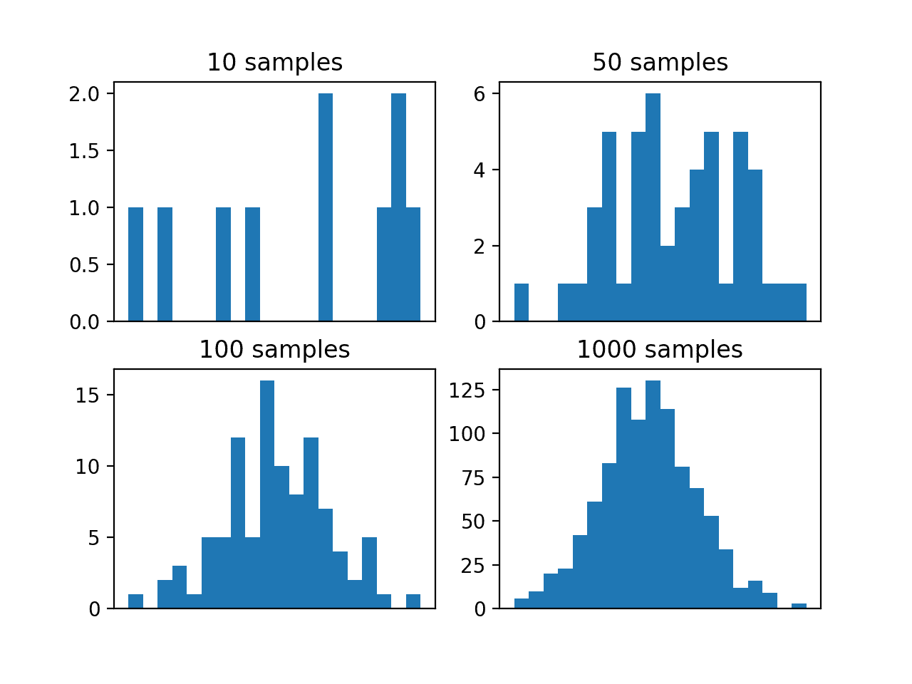
In this case, we will have a function that defines the probability distribution of a random variable. We will use a Gaussian distribution with a mean of 50 and a standard deviation of 5 and draw random samples from this distribution.
Let’s pretend we don’t know the form of the probability distribution for this random variable and we want to sample the function to get an idea of the probability density. We can draw a sample of a given size and plot a histogram to estimate the density.
The normal() NumPy function can be used to randomly draw samples from a Gaussian distribution with the specified mean (mu), standard deviation (sigma), and sample size.
To make the example more interesting, we will repeat this experiment four times with different sized samples. We would expect that as the size of the sample is increased, the probability density will better approximate the true density of the target function, given the law of large numbers.
The complete example is listed below.
1
2
3
4
5
6
7
8
9
10
11
12
13
14
15
16
17
18
# example of effect of size on monte carlo sample
from numpy.random import normal
from matplotlib import pyplot
# define the distribution
mu=50
sigma=5
# generate monte carlo samples of differing size
sizes=[10,50,100,1000]
foriinrange(len(sizes)):
# generate sample
sample=normal(mu,sigma,sizes[i])
# plot histogram of sample
pyplot.subplot(2,2,i+1)
pyplot.hist(sample,bins=20)
pyplot.title('%d samples'%sizes[i])
pyplot.xticks([])
# show the plot
pyplot.show()
Running the example creates four differently sized samples and plots a histogram for each.
We can see that the small sample sizes of 10 and 50 do not effectively capture the density of the target function. We can see that 100 samples is better, but it is not until 1,000 samples that we clearly see the familiar bell-shape of the Gaussian probability distribution.
This highlights the need to draw many samples, even for a simple random variable, and the benefit of increased accuracy of the approximation with the number of samples drawn.
Histogram Plots of Differently Sized Monte Carlo Samples From the Target Function
Further Reading
This section provides more resources on the topic if you are looking to go deeper.
In this post, you discovered Monte Carlo methods for sampling probability distributions.
Specifically, you learned:
Often, we cannot calculate a desired quantity in probability, but we can define the probability distributions for the random variables directly or indirectly.
Monte Carlo sampling a class of methods for randomly sampling from a probability distribution.
Monte Carlo sampling provides the foundation for many machine learning methods such as resampling, hyperparameter tuning, and ensemble learning.
Do you have any questions?
Ask your questions in the comments below and I will do my best to answer.
It provides self-study tutorials and end-to-end projects on: Bayes Theorem, Bayesian Optimization, Distributions, Maximum Likelihood, Cross-Entropy, Calibrating Models
and much more...
I am interested in taking this crash course to better understand Probability and Monte Carlo Simulation using Python. I am tasked with invalidating a Risk Model for my organization. with this validation, I would like to have a better understanding of what I am doing and what the step by step process of understanding the Monte Carlo Simulation. I have a degree in Computer Science and have knowledge of R and Python. I have purchased your E-books and have not really completed any of the assignments and I needed to take a leap of faith to complete an assignment. I think this is my leap of faith.
I have to do MC uncertainty test to see the ANN prediction how well performing in ‘R’?
So my questions as follows:
1) for the randome sampling for MC simulation: should I aspect to find mu, sigma etc from actual value OR predicted value by ANN model
2) how to decide number of size? And in each size the no of sample as here you selected 10, 50, 100, 1000
3) in last, as you described that the well shaped distribution graph will be preferable to report I.e. well explained sample size SO in my case also the same sample size need to be model for the ANN to see the its predictive compatibility?
Sorry if my question is confusing to you. My aim is to use MC to analyze the uncertainty of ANN prediction performance.
Dear Dr Jason,
In the above example you simulated a normal distribution for various sample sizes.
I have question about this.
While the shape of the histograms of the smaller sampled simulations did not resemble the normal distribution, is there a statistical test to determining whether the small sampled set(s) did come from a normal distribution for example using the K-S test or Shapiro-Wilks test OR even using Entropy?
I have another question about Monte Carlo simulation:
I recall in an undergraduate unit doing an exercise in Monte Carlo simulation. For example generating 1000 samples from the uniform distribution and determining the proportion of samples lying within the unit circle over the total number of generated points. The result is an approximation of pi = 3.141.
Is this application of Monte Carlo simulation used in machine learning?
Dear Dr Jason,
I had a goo at the “a gentle introduction to normality tests in python”.
There was the visual test using the qqplot and the three tests.
I generated small samples of size 50 and 20 from the normal distribution. Using the qqplot, there was ‘symmetry’ with half the values above and half the values below the ‘theoretical’ test.
The graphical plot is not the be all and end all of visual display.
As you said in regards to tests, you suggest doing all three numerical statistical tests.
For your information, the statistical tests for a sample size of 20 and 50 indicated that despite the data not visually looking normal, all numerical Shapiro-Wilk, Anderson and D’Agostino indicated the the sample size were likely to be from a normal distribution. All p values > alpha.
I am a bit confused from where the values of the sample come from ?
For example, supposing I have trained a model using using RNN, and I want to predict the next day, based on the last 5 observation (eg. [10, 30, 50, 5, 4]).
Using a Poisson Likehood and create the equivalent of Monte Carlo trace in order that in the end I can calculate e.g. quantiles of the output distribution or assess uncertainty of the predictions.
i have a question about neutron transport in a multi-regions slab, if you have a flow chart or a figure that illustrates the steps of the process, i am trying to program it using python but I could not
I’m trying to use Markov Chain Monte Carlo for entanglement swapping to realize a long distance quantum communication, do you think that MCMC can increase the bite rate between the end of a node of a channel and the beginning of the other
and to make the question more clear here i quote from an article that says:
“However, the distances achievable with quantum relays are still
limited. Th e reason is that in order to be able to swap the entanglement
of pair A–B and of pair B–C to A–C, the entanglement between the
pairs A–B and B–C has to be established fi rst. However, the probability
that all photons propagate between A and B and between B and C is
precisely the same probability that a photon propagates from A directly
to C. Hence, there is no hope that entanglement swapping by itself helps
to increase the bit rate.”
Many thanks for this wonderful tutorial. I have a question.
How would one do a MC sampling of a modified normal distribution such as f(x)*normal distribution where f(x) can be any function such as x**2 or something.
Many thanks for this wonderful tutorial. I have a question.
Suppose I have a set of data and a function f(x). Using that set of data, I plot a histogram. If the histogram is somewhat well behaved, I can approximately figure out the probability density function p(x) and use that to compute \int p(x)*f(x) which is the end goal.
When the histogram is not well behaved and it is almost impossible for one to approximate a PDF, p(x), how would one go about numerically computing \int p(x)*f(x) given the data and f(x) only?
Many thanks for your reply. I really appreciate it!
This empirical distribution function works well. However, when it comes to integration (which is the final goal), I have no idea how to do it.
Suppose I use the empirical distribution, I am able to plot the curve that results. How do I then take that output, multiply it with f(x) and then integrate it?
I believe you can read off individual values (e.g. P(x) or x for P, but I don’t think it gives more advanced tools than that. I recommend checking the API.
Thanks for the breif article. I would like to summariye few things I have learnt from reading lot of material over the days with regards to the problem i am looking to solve.Lets say I have bounds for two input parameters (min,max) , and I have no clue regarding the underlying distribution the parameters follows. So from what I understood is i will carry out goodness of fit test to confirm my assumptions regarding input parameters and then go ahead with monte carlo simulations. To check number of iterations required I would then check for the variance after each simulation? or is there any other way around?
Also when exactly sampling techniques are used?
And how to say the output distribution is the best for my model? perform another goodness of fit test?
And when to use sampling method, markov method or particle filter method? or how can I eliminate the posibilty of solving my model using diffrent methods?
Also using diffrent sampling techniques also classify as a method?
Perhaps start with something really simple, like sample your domain on a grid and create some plots of each variable to get a feeling for the distributions and relationships.
Dear Dr.Brownlee
Hi,
As you know, for deep learning modeling, a lot of data is needed. If there are limited data for a region/problem,could I increase the number of points (data) by a technique (e.g. Monte Carlo method) and then use deep learning? In other words, is the deep learning model reliable in this condition?
In many engineering problems often enough data aren’t available, therefore application of deep learning is a challenge.
Thanks for your help.
How much data you needed really depends on the problem you are going to solve. One technique is to use bootstrapping to amplify the data set (see https://machinelearningmastery.com/a-gentle-introduction-to-the-bootstrap-method/ for an introduction). For image processing tasks, people has various methods to augment the data, such as rotating the image a bit, flip it, tune the color, etc. You might even think of a smart way to produce data by simulation. Hope this can ignite your thought on how to solve your problem.


I am interested in taking this crash course to better understand Probability and Monte Carlo Simulation using Python. I am tasked with invalidating a Risk Model for my organization. with this validation, I would like to have a better understanding of what I am doing and what the step by step process of understanding the Monte Carlo Simulation. I have a degree in Computer Science and have knowledge of R and Python. I have purchased your E-books and have not really completed any of the assignments and I needed to take a leap of faith to complete an assignment. I think this is my leap of faith.
Hang in there Gladys.
Monte Carlo simulation is very simple at the core. It’s just a tool with a fancy name.
Focus on what it can teach you about your specific model.
Great work for learners.
Thanks!
Dear Dr. Jason
I have to do MC uncertainty test to see the ANN prediction how well performing in ‘R’?
So my questions as follows:
1) for the randome sampling for MC simulation: should I aspect to find mu, sigma etc from actual value OR predicted value by ANN model
2) how to decide number of size? And in each size the no of sample as here you selected 10, 50, 100, 1000
3) in last, as you described that the well shaped distribution graph will be preferable to report I.e. well explained sample size SO in my case also the same sample size need to be model for the ANN to see the its predictive compatibility?
Sorry if my question is confusing to you. My aim is to use MC to analyze the uncertainty of ANN prediction performance.
best regards
Suraj
You are finding mu and sigma in the prediction error.
Perhaps keep it small to avoid computational cost, e.g. 30.
Would you be comfortable sharing a bit more of your methods? I am working on something similar and finding some difficulty.
Dear Dr Jason,
In the above example you simulated a normal distribution for various sample sizes.
I have question about this.
While the shape of the histograms of the smaller sampled simulations did not resemble the normal distribution, is there a statistical test to determining whether the small sampled set(s) did come from a normal distribution for example using the K-S test or Shapiro-Wilks test OR even using Entropy?
I have another question about Monte Carlo simulation:
I recall in an undergraduate unit doing an exercise in Monte Carlo simulation. For example generating 1000 samples from the uniform distribution and determining the proportion of samples lying within the unit circle over the total number of generated points. The result is an approximation of pi = 3.141.
Is this application of Monte Carlo simulation used in machine learning?
Thank you,
Anthony of Sydney
Yes, one of these tests:
https://machinelearningmastery.com/a-gentle-introduction-to-normality-tests-in-python/
Yes, it’s a great use of the method to approximate a quantity.
Dear Dr Jason,
I had a goo at the “a gentle introduction to normality tests in python”.
There was the visual test using the qqplot and the three tests.
I generated small samples of size 50 and 20 from the normal distribution. Using the qqplot, there was ‘symmetry’ with half the values above and half the values below the ‘theoretical’ test.
The graphical plot is not the be all and end all of visual display.
As you said in regards to tests, you suggest doing all three numerical statistical tests.
For your information, the statistical tests for a sample size of 20 and 50 indicated that despite the data not visually looking normal, all numerical Shapiro-Wilk, Anderson and D’Agostino indicated the the sample size were likely to be from a normal distribution. All p values > alpha.
Thank you,
Anthony of Sydney
Very nice work!
Hi Jason,
Thank you for your post.
I am a bit confused from where the values of the sample come from ?
For example, supposing I have trained a model using using RNN, and I want to predict the next day, based on the last 5 observation (eg. [10, 30, 50, 5, 4]).
Using a Poisson Likehood and create the equivalent of Monte Carlo trace in order that in the end I can calculate e.g. quantiles of the output distribution or assess uncertainty of the predictions.
In that case, you could have an ensemble of models, each making a prediction and sampling the prediction space.
Or one model with small randomness added to the input and in turn sample the prediction space.
i have a question about neutron transport in a multi-regions slab, if you have a flow chart or a figure that illustrates the steps of the process, i am trying to program it using python but I could not
Sorry, I do not.
Dear Dr Jason
I’m trying to use Markov Chain Monte Carlo for entanglement swapping to realize a long distance quantum communication, do you think that MCMC can increase the bite rate between the end of a node of a channel and the beginning of the other
and to make the question more clear here i quote from an article that says:
“However, the distances achievable with quantum relays are still
limited. Th e reason is that in order to be able to swap the entanglement
of pair A–B and of pair B–C to A–C, the entanglement between the
pairs A–B and B–C has to be established fi rst. However, the probability
that all photons propagate between A and B and between B and C is
precisely the same probability that a photon propagates from A directly
to C. Hence, there is no hope that entanglement swapping by itself helps
to increase the bit rate.”
Thank you
I don’t know, sorry.
Hi Jason,
Many thanks for this wonderful tutorial. I have a question.
How would one do a MC sampling of a modified normal distribution such as f(x)*normal distribution where f(x) can be any function such as x**2 or something.
Many thanks,
Ameir
Why not sample the function directly?
If that is a problem, why not use an empirical distribution:
https://machinelearningmastery.com/empirical-distribution-function-in-python/
Hi Jason,
Many thanks for this wonderful tutorial. I have a question.
Suppose I have a set of data and a function f(x). Using that set of data, I plot a histogram. If the histogram is somewhat well behaved, I can approximately figure out the probability density function p(x) and use that to compute \int p(x)*f(x) which is the end goal.
When the histogram is not well behaved and it is almost impossible for one to approximate a PDF, p(x), how would one go about numerically computing \int p(x)*f(x) given the data and f(x) only?
See this:
https://machinelearningmastery.com/empirical-distribution-function-in-python/
Hi Jason,
Many thanks for your reply. I really appreciate it!
This empirical distribution function works well. However, when it comes to integration (which is the final goal), I have no idea how to do it.
Suppose I use the empirical distribution, I am able to plot the curve that results. How do I then take that output, multiply it with f(x) and then integrate it?
Many thanks,
Ameir
I believe you can read off individual values (e.g. P(x) or x for P, but I don’t think it gives more advanced tools than that. I recommend checking the API.
Hi Jason,
Great article – very clear and informative. But thought you might want to know that the photo is from Vernazza in Italy, not Monte Carlo!
Thanks!
Hey Jason,
Thanks for the breif article. I would like to summariye few things I have learnt from reading lot of material over the days with regards to the problem i am looking to solve.Lets say I have bounds for two input parameters (min,max) , and I have no clue regarding the underlying distribution the parameters follows. So from what I understood is i will carry out goodness of fit test to confirm my assumptions regarding input parameters and then go ahead with monte carlo simulations. To check number of iterations required I would then check for the variance after each simulation? or is there any other way around?
Also when exactly sampling techniques are used?
And how to say the output distribution is the best for my model? perform another goodness of fit test?
And when to use sampling method, markov method or particle filter method? or how can I eliminate the posibilty of solving my model using diffrent methods?
Also using diffrent sampling techniques also classify as a method?
Faithfull Student
Biddappa
Perhaps start with something really simple, like sample your domain on a grid and create some plots of each variable to get a feeling for the distributions and relationships.
what are some comparative techniques to the monte carlo technique if i am trying to decide which to choose?
Perhaps other sampling algorithms:
https://en.wikipedia.org/wiki/Markov_chain_Monte_Carlo
Dear Dr.Brownlee
Hi,
As you know, for deep learning modeling, a lot of data is needed. If there are limited data for a region/problem,could I increase the number of points (data) by a technique (e.g. Monte Carlo method) and then use deep learning? In other words, is the deep learning model reliable in this condition?
In many engineering problems often enough data aren’t available, therefore application of deep learning is a challenge.
Thanks for your help.
How much data you needed really depends on the problem you are going to solve. One technique is to use bootstrapping to amplify the data set (see https://machinelearningmastery.com/a-gentle-introduction-to-the-bootstrap-method/ for an introduction). For image processing tasks, people has various methods to augment the data, such as rotating the image a bit, flip it, tune the color, etc. You might even think of a smart way to produce data by simulation. Hope this can ignite your thought on how to solve your problem.
Please specify in the above picture thet the landscape you published is not Monte Carlo but Vernazza in Italy. Thanks.
Thank you for the feedback Pierfranco!