A Gentle Introduction to Expectation-Maximization (EM Algorithm)

Maximum likelihood estimation is an approach to density estimation for a dataset by searching across probability distributions and their parameters.

It is a general and effective approach that underlies many machine learning algorithms, although it requires that the training dataset is complete, e.g. all relevant interacting random variables are present. Maximum likelihood becomes intractable if there are variables that interact with those in the dataset but were hidden or not observed, so-called latent variables.

The expectation-maximization algorithm is an approach for performing maximum likelihood estimation in the presence of latent variables. It does this by first estimating the values for the latent variables, then optimizing the model, then repeating these two steps until convergence. It is an effective and general approach and is most commonly used for density estimation with missing data, such as clustering algorithms like the Gaussian Mixture Model.

In this post, you will discover the expectation-maximization algorithm.

After reading this post, you will know:

• Maximum likelihood estimation is challenging on data in the presence of latent variables.
• Expectation maximization provides an iterative solution to maximum likelihood estimation with latent variables.
• Gaussian mixture models are an approach to density estimation where the parameters of the distributions are fit using the expectation-maximization algorithm.

Kick-start your project with my new book Probability for Machine Learning, including step-by-step tutorials and the Python source code files for all examples.

Let’s get started.

• Update Nov/2019: Fixed typo in code comment (thanks Daniel)

A Gentle Introduction to Expectation Maximization (EM Algorithm)
Photo by valcker, some rights reserved.

Overview

This tutorial is divided into four parts; they are:

1. Problem of Latent Variables for Maximum Likelihood
2. Expectation-Maximization Algorithm
3. Gaussian Mixture Model and the EM Algorithm
4. Example of Gaussian Mixture Model

Problem of Latent Variables for Maximum Likelihood

A common modeling problem involves how to estimate a joint probability distribution for a dataset.

Density estimation involves selecting a probability distribution function and the parameters of that distribution that best explain the joint probability distribution of the observed data.

There are many techniques for solving this problem, although a common approach is called maximum likelihood estimation, or simply “maximum likelihood.”

Maximum Likelihood Estimation involves treating the problem as an optimization or search problem, where we seek a set of parameters that results in the best fit for the joint probability of the data sample.

A limitation of maximum likelihood estimation is that it assumes that the dataset is complete, or fully observed. This does not mean that the model has access to all data; instead, it assumes that all variables that are relevant to the problem are present.

This is not always the case. There may be datasets where only some of the relevant variables can be observed, and some cannot, and although they influence other random variables in the dataset, they remain hidden.

More generally, these unobserved or hidden variables are referred to as latent variables.

Many real-world problems have hidden variables (sometimes called latent variables), which are not observable in the data that are available for learning.

— Page 816, Artificial Intelligence: A Modern Approach, 3rd edition, 2009.

Conventional maximum likelihood estimation does not work well in the presence of latent variables.

… if we have missing data and/or latent variables, then computing the [maximum likelihood] estimate becomes hard.

— Page 349, Machine Learning: A Probabilistic Perspective, 2012.

Instead, an alternate formulation of maximum likelihood is required for searching for the appropriate model parameters in the presence of latent variables.

The Expectation-Maximization algorithm is one such approach.

Expectation-Maximization Algorithm

The Expectation-Maximization Algorithm, or EM algorithm for short, is an approach for maximum likelihood estimation in the presence of latent variables.

A general technique for finding maximum likelihood estimators in latent variable models is the expectation-maximization (EM) algorithm.

— Page 424, Pattern Recognition and Machine Learning, 2006.

The EM algorithm is an iterative approach that cycles between two modes. The first mode attempts to estimate the missing or latent variables, called the estimation-step or E-step. The second mode attempts to optimize the parameters of the model to best explain the data, called the maximization-step or M-step.

• E-Step. Estimate the missing variables in the dataset.
• M-Step. Maximize the parameters of the model in the presence of the data.

The EM algorithm can be applied quite widely, although is perhaps most well known in machine learning for use in unsupervised learning problems, such as density estimation and clustering.

Perhaps the most discussed application of the EM algorithm is for clustering with a mixture model.

Gaussian Mixture Model and the EM Algorithm

A mixture model is a model comprised of an unspecified combination of multiple probability distribution functions.

A statistical procedure or learning algorithm is used to estimate the parameters of the probability distributions to best fit the density of a given training dataset.

The Gaussian Mixture Model, or GMM for short, is a mixture model that uses a combination of Gaussian (Normal) probability distributions and requires the estimation of the mean and standard deviation parameters for each.

There are many techniques for estimating the parameters for a GMM, although a maximum likelihood estimate is perhaps the most common.

Consider the case where a dataset is comprised of many points that happen to be generated by two different processes. The points for each process have a Gaussian probability distribution, but the data is combined and the distributions are similar enough that it is not obvious to which distribution a given point may belong.

The processes used to generate the data point represents a latent variable, e.g. process 0 and process 1. It influences the data but is not observable. As such, the EM algorithm is an appropriate approach to use to estimate the parameters of the distributions.

In the EM algorithm, the estimation-step would estimate a value for the process latent variable for each data point, and the maximization step would optimize the parameters of the probability distributions in an attempt to best capture the density of the data. The process is repeated until a good set of latent values and a maximum likelihood is achieved that fits the data.

• E-Step. Estimate the expected value for each latent variable.
• M-Step. Optimize the parameters of the distribution using maximum likelihood.

We can imagine how this optimization procedure could be constrained to just the distribution means, or generalized to a mixture of many different Gaussian distributions.

Example of Gaussian Mixture Model

We can make the application of the EM algorithm to a Gaussian Mixture Model concrete with a worked example.

First, let’s contrive a problem where we have a dataset where points are generated from one of two Gaussian processes. The points are one-dimensional, the mean of the first distribution is 20, the mean of the second distribution is 40, and both distributions have a standard deviation of 5.

We will draw 3,000 points from the first process and 7,000 points from the second process and mix them together.

We can then plot a histogram of the points to give an intuition for the dataset. We expect to see a bimodal distribution with a peak for each of the means of the two distributions.

The complete example is listed below.

Running the example creates the dataset and then creates a histogram plot for the data points.

The plot clearly shows the expected bimodal distribution with a peak for the first process around 20 and a peak for the second process around 40.

We can see that for many of the points in the middle of the two peaks that it is ambiguous as to which distribution they were drawn from.

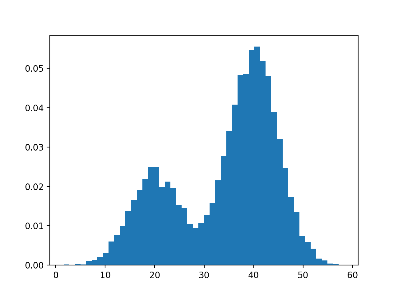
Histogram of Dataset Constructed From Two Different Gaussian Processes

We can model the problem of estimating the density of this dataset using a Gaussian Mixture Model.

The GaussianMixture scikit-learn class can be used to model this problem and estimate the parameters of the distributions using the expectation-maximization algorithm.

The class allows us to specify the suspected number of underlying processes used to generate the data via the n_components argument when defining the model. We will set this to 2 for the two processes or distributions.

If the number of processes was not known, a range of different numbers of components could be tested and the model with the best fit could be chosen, where models could be evaluated using scores such as Akaike or Bayesian Information Criterion (AIC or BIC).

There are also many ways we can configure the model to incorporate other information we may know about the data, such as how to estimate initial values for the distributions. In this case, we will randomly guess the initial parameters, by setting the init_params argument to ‘random’.

Once the model is fit, we can access the learned parameters via arguments on the model, such as the means, covariances, mixing weights, and more.

More usefully, we can use the fit model to estimate the latent parameters for existing and new data points.

For example, we can estimate the latent variable for the points in the training dataset and we would expect the first 3,000 points to belong to one process (e.g. value=1) and the next 7,000 data points to belong to a different process (e.g. value=0).

Tying all of this together, the complete example is listed below.

Running the example fits the Gaussian mixture model on the prepared dataset using the EM algorithm. Once fit, the model is used to predict the latent variable values for the examples in the training dataset.

Note: Your results may vary given the stochastic nature of the algorithm or evaluation procedure, or differences in numerical precision. Consider running the example a few times and compare the average outcome.

In this case, we can see that at least for the first few and last few examples in the dataset, that the model mostly predicts the correct value for the latent variable. It’s a generally challenging problem and it is expected that the points between the peaks of the distribution will remain ambiguous and assigned to one process or another holistically.

Further Reading

This section provides more resources on the topic if you are looking to go deeper.

Books

• Section 8.5 The EM Algorithm, The Elements of Statistical Learning, 2016.
• Chapter 9 Mixture Models and EM, Pattern Recognition and Machine Learning, 2006.
• Section 6.12 The EM Algorithm, Machine Learning, 1997.
• Chapter 11 Mixture models and the EM algorithm, Machine Learning: A Probabilistic Perspective, 2012.
• Section 9.3 Clustering And Probability Density Estimation, Data Mining: Practical Machine Learning Tools and Techniques, 4th edition, 2016.
• Section 20.3 Learning With Hidden Variables: The EM Algorithm, Artificial Intelligence: A Modern Approach, 3rd edition, 2009.

API

• Gaussian mixture models, scikit-learn API.
• sklearn.mixture.GaussianMixture API.

Articles

• Maximum likelihood estimation, Wikipedia.
• Expectation-maximization algorithm, Wikipedia.
• Mixture model, Wikipedia.

Summary

In this post, you discovered the expectation-maximization algorithm.

Specifically, you learned:

• Maximum likelihood estimation is challenging on data in the presence of latent variables.
• Expectation maximization provides an iterative solution to maximum likelihood estimation with latent variables.
• Gaussian mixture models are an approach to density estimation where the parameters of the distributions are fit using the expectation-maximization algorithm.

Do you have any questions?
Ask your questions in the comments below and I will do my best to answer.

Get a Handle on Probability for Machine Learning!

Develop Your Understanding of Probability

...with just a few lines of python code

Discover how in my new Ebook:
Probability for Machine Learning

It provides self-study tutorials and end-to-end projects on:
Bayes Theorem, Bayesian Optimization, Distributions, Maximum Likelihood, Cross-Entropy, Calibrating Models
and much more...

Finally Harness Uncertainty in Your Projects

Skip the Academics. Just Results.

See What's Inside