
Numerical input variables may have a highly skewed or non-standard distribution.
This could be caused by outliers in the data, multi-modal distributions, highly exponential distributions, and more.
Many machine learning algorithms prefer or perform better when numerical input variables have a standard probability distribution.
The discretization transform provides an automatic way to change a numeric input variable to have a different data distribution, which in turn can be used as input to a predictive model.
In this tutorial, you will discover how to use discretization transforms to map numerical values to discrete categories for machine learning
After completing this tutorial, you will know:
- Many machine learning algorithms prefer or perform better when numerical with non-standard probability distributions are made discrete.
- Discretization transforms are a technique for transforming numerical input or output variables to have discrete ordinal labels.
- How to use the KBinsDiscretizer to change the structure and distribution of numeric variables to improve the performance of predictive models.
Kick-start your project with my new book Data Preparation for Machine Learning, including step-by-step tutorials and the Python source code files for all examples.
Let’s get started.
How to Use Discretization Transforms for Machine Learning
Photo by Kate Russell, some rights reserved.
Tutorial Overview
This tutorial is divided into six parts; they are:
- Change Data Distribution
- Discretization Transforms
- Sonar Dataset
- Uniform Discretization Transform
- K-means Discretization Transform
- Quantile Discretization Transform
Change Data Distribution
Some machine learning algorithms may prefer or require categorical or ordinal input variables, such as some decision tree and rule-based algorithms.
Some classification and clustering algorithms deal with nominal attributes only and cannot handle ones measured on a numeric scale.
— Page 296, Data Mining: Practical Machine Learning Tools and Techniques, 4th edition, 2016.
Further, the performance of many machine learning algorithms degrades for variables that have non-standard probability distributions.
This applies both to real-valued input variables in the case of classification and regression tasks, and real-valued target variables in the case of regression tasks.
Some input variables may have a highly skewed distribution, such as an exponential distribution where the most common observations are bunched together. Some input variables may have outliers that cause the distribution to be highly spread.
These concerns and others, like non-standard distributions and multi-modal distributions, can make a dataset challenging to model with a range of machine learning models.
As such, it is often desirable to transform each input variable to have a standard probability distribution.
One approach is to use transform of the numerical variable to have a discrete probability distribution where each numerical value is assigned a label and the labels have an ordered (ordinal) relationship.
This is called a binning or a discretization transform and can improve the performance of some machine learning models for datasets by making the probability distribution of numerical input variables discrete.
Want to Get Started With Data Preparation?
Take my free 7-day email crash course now (with sample code).
Click to sign-up and also get a free PDF Ebook version of the course.
Discretization Transforms
A discretization transform will map numerical variables onto discrete values.
Binning, also known as categorization or discretization, is the process of translating a quantitative variable into a set of two or more qualitative buckets (i.e., categories).
— Page 129, Feature Engineering and Selection, 2019.
Values for the variable are grouped together into discrete bins and each bin is assigned a unique integer such that the ordinal relationship between the bins is preserved.
The use of bins is often referred to as binning or k-bins, where k refers to the number of groups to which a numeric variable is mapped.
The mapping provides a high-order ranking of values that can smooth out the relationships between observations. The transformation can be applied to each numeric input variable in the training dataset and then provided as input to a machine learning model to learn a predictive modeling task.
The determination of the bins must be included inside of the resampling process.
— Page 132, Feature Engineering and Selection, 2019.
Different methods for grouping the values into k discrete bins can be used; common techniques include:
- Uniform: Each bin has the same width in the span of possible values for the variable.
- Quantile: Each bin has the same number of values, split based on percentiles.
- Clustered: Clusters are identified and examples are assigned to each group.
The discretization transform is available in the scikit-learn Python machine learning library via the KBinsDiscretizer class.
The “strategy” argument controls the manner in which the input variable is divided, as either “uniform,” “quantile,” or “kmeans.”
The “n_bins” argument controls the number of bins that will be created and must be set based on the choice of strategy, e.g. “uniform” is flexible, “quantile” must have a “n_bins” less than the number of observations or sensible percentiles, and “kmeans” must use a value for the number of clusters that can be reasonably found.
The “encode” argument controls whether the transform will map each value to an integer value by setting “ordinal” or a one-hot encoding “onehot.” An ordinal encoding is almost always preferred, although a one-hot encoding may allow a model to learn non-ordinal relationships between the groups, such as in the case of k-means clustering strategy.
We can demonstrate the KBinsDiscretizer with a small worked example. We can generate a sample of random Gaussian numbers. The KBinsDiscretizer can then be used to convert the floating values into fixed number of discrete categories with an ranked ordinal relationship.
The complete example is listed below.
|
1 2 3 4 5 6 7 8 9 10 11 12 13 14 15 16 17 18 19 |
# demonstration of the discretization transform from numpy.random import randn from sklearn.preprocessing import KBinsDiscretizer from matplotlib import pyplot # generate gaussian data sample data = randn(1000) # histogram of the raw data pyplot.hist(data, bins=25) pyplot.show() # reshape data to have rows and columns data = data.reshape((len(data),1)) # discretization transform the raw data kbins = KBinsDiscretizer(n_bins=10, encode='ordinal', strategy='uniform') data_trans = kbins.fit_transform(data) # summarize first few rows print(data_trans[:10, :]) # histogram of the transformed data pyplot.hist(data_trans, bins=10) pyplot.show() |
Running the example first creates a sample of 1,000 random Gaussian floating-point values and plots the data as a histogram.
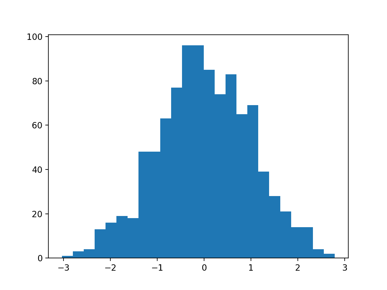
Histogram of Data With a Gaussian Distribution
Next the KBinsDiscretizer is used to map the numerical values to categorical values. We configure the transform to create 10 categories (0 to 9), to output the result in ordinal format (integers) and to divide the range of the input data uniformly.
A sample of the transformed data is printed, clearly showing the integer format of the data as expected.
|
1 2 3 4 5 6 7 8 9 10 |
[[5.] [3.] [2.] [6.] [7.] [5.] [3.] [4.] [4.] [2.]] |
Finally, a histogram is created showing the 10 discrete categories and how the observations are distributed across these groups, following the same pattern as the original data with a Gaussian shape.
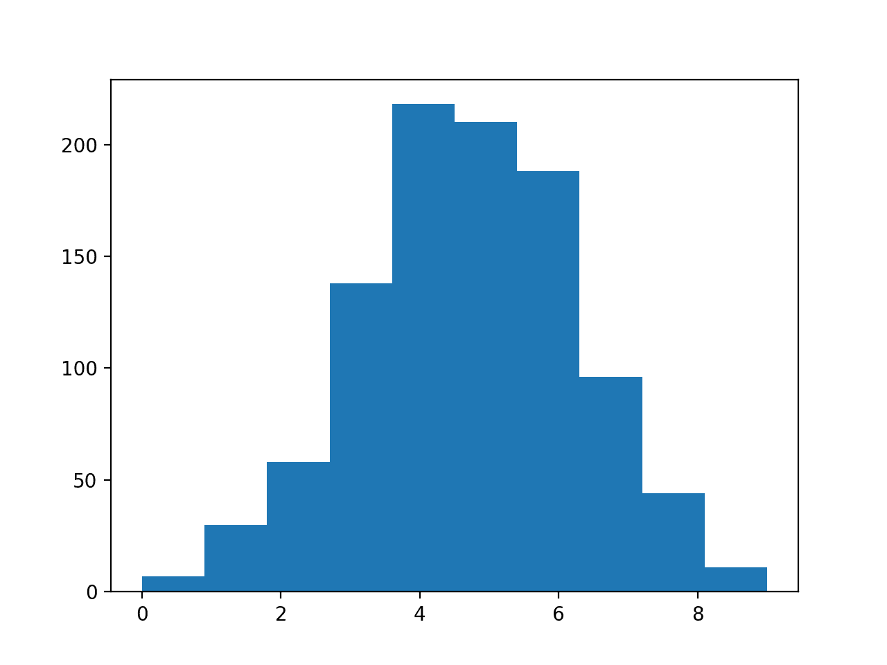
Histogram of Transformed Data With Discrete Categories
In the following sections will take a closer look at how to use the discretization transform on a real dataset.
Next, let’s introduce the dataset.
Sonar Dataset
The sonar dataset is a standard machine learning dataset for binary classification.
It involves 60 real-valued inputs and a two-class target variable. There are 208 examples in the dataset and the classes are reasonably balanced.
A baseline classification algorithm can achieve a classification accuracy of about 53.4 percent using repeated stratified 10-fold cross-validation. Top performance on this dataset is about 88 percent using repeated stratified 10-fold cross-validation.
The dataset describes radar returns of rocks or simulated mines.
You can learn more about the dataset from here:
No need to download the dataset; we will download it automatically from our worked examples.
First, let’s load and summarize the dataset. The complete example is listed below.
|
1 2 3 4 5 6 7 8 9 10 11 12 13 14 |
# load and summarize the sonar dataset from pandas import read_csv from pandas.plotting import scatter_matrix from matplotlib import pyplot # Load dataset url = "https://raw.githubusercontent.com/jbrownlee/Datasets/master/sonar.csv" dataset = read_csv(url, header=None) # summarize the shape of the dataset print(dataset.shape) # summarize each variable print(dataset.describe()) # histograms of the variables dataset.hist() pyplot.show() |
Running the example first summarizes the shape of the loaded dataset.
This confirms the 60 input variables, one output variable, and 208 rows of data.
A statistical summary of the input variables is provided showing that values are numeric and range approximately from 0 to 1.
|
1 2 3 4 5 6 7 8 9 10 11 12 |
(208, 61) 0 1 2 ... 57 58 59 count 208.000000 208.000000 208.000000 ... 208.000000 208.000000 208.000000 mean 0.029164 0.038437 0.043832 ... 0.007949 0.007941 0.006507 std 0.022991 0.032960 0.038428 ... 0.006470 0.006181 0.005031 min 0.001500 0.000600 0.001500 ... 0.000300 0.000100 0.000600 25% 0.013350 0.016450 0.018950 ... 0.003600 0.003675 0.003100 50% 0.022800 0.030800 0.034300 ... 0.005800 0.006400 0.005300 75% 0.035550 0.047950 0.057950 ... 0.010350 0.010325 0.008525 max 0.137100 0.233900 0.305900 ... 0.044000 0.036400 0.043900 [8 rows x 60 columns] |
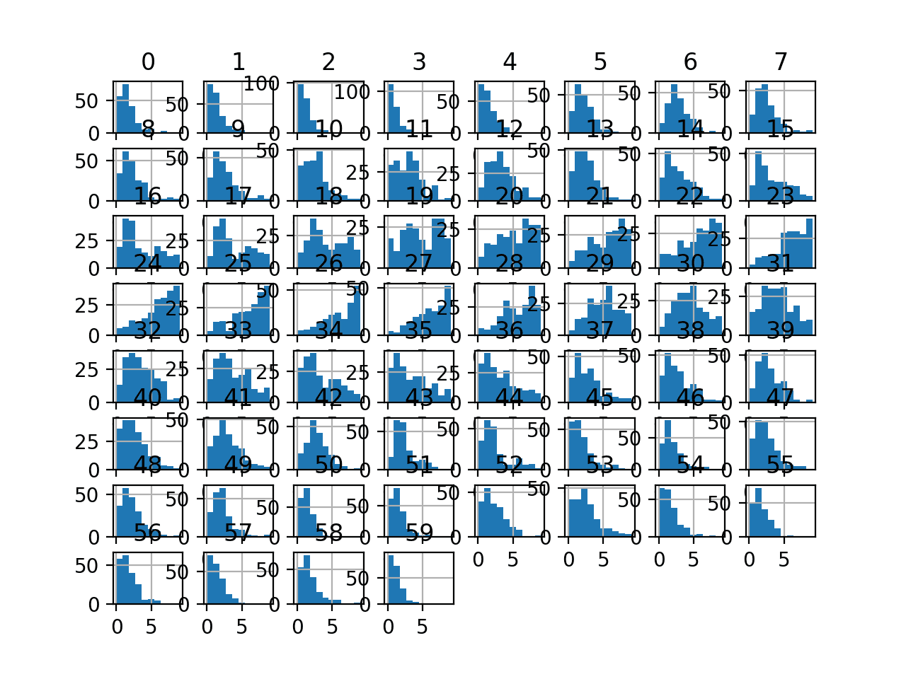
Finally, a histogram is created for each input variable.
If we ignore the clutter of the plots and focus on the histograms themselves, we can see that many variables have a skewed distribution.
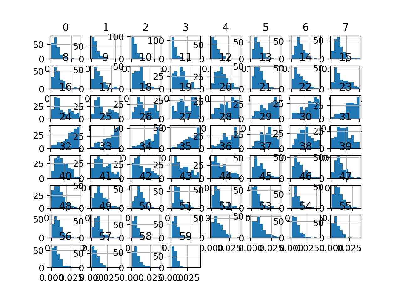
Histogram Plots of Input Variables for the Sonar Binary Classification Dataset
Next, let’s fit and evaluate a machine learning model on the raw dataset.
We will use a k-nearest neighbor algorithm with default hyperparameters and evaluate it using repeated stratified k-fold cross-validation.
The complete example is listed below.
|
1 2 3 4 5 6 7 8 9 10 11 12 13 14 15 16 17 18 19 20 21 22 23 24 25 |
# evaluate knn on the raw sonar dataset from numpy import mean from numpy import std from pandas import read_csv from sklearn.model_selection import cross_val_score from sklearn.model_selection import RepeatedStratifiedKFold from sklearn.neighbors import KNeighborsClassifier from sklearn.preprocessing import LabelEncoder from matplotlib import pyplot # load dataset url = "https://raw.githubusercontent.com/jbrownlee/Datasets/master/sonar.csv" dataset = read_csv(url, header=None) data = dataset.values # separate into input and output columns X, y = data[:, :-1], data[:, -1] # ensure inputs are floats and output is an integer label X = X.astype('float32') y = LabelEncoder().fit_transform(y.astype('str')) # define and configure the model model = KNeighborsClassifier() # evaluate the model cv = RepeatedStratifiedKFold(n_splits=10, n_repeats=3, random_state=1) n_scores = cross_val_score(model, X, y, scoring='accuracy', cv=cv, n_jobs=-1, error_score='raise') # report model performance print('Accuracy: %.3f (%.3f)' % (mean(n_scores), std(n_scores))) |
Running the example evaluates a KNN model on the raw sonar dataset.
Note: Your results may vary given the stochastic nature of the algorithm or evaluation procedure, or differences in numerical precision. Consider running the example a few times and compare the average outcome.
We can see that the model achieved a mean classification accuracy of about 79.7 percent, showing that it has skill (better than 53.4 percent) and is in the ball-park of good performance (88 percent).
|
1 |
Accuracy: 0.797 (0.073) |
Next, let’s explore a uniform discretization transform of the dataset.
Uniform Discretization Transform
A uniform discretization transform will preserve the probability distribution of each input variable but will make it discrete with the specified number of ordinal groups or labels.
We can apply the uniform discretization transform using the KBinsDiscretizer class and setting the “strategy” argument to “uniform.” We must also set the desired number of bins set via the “n_bins” argument; in this case, we will use 10.
Once defined, we can call the fit_transform() function and pass it our dataset to create a quantile transformed version of our dataset.
|
1 2 3 4 |
... # perform a uniform discretization transform of the dataset trans = KBinsDiscretizer(n_bins=10, encode='ordinal', strategy='uniform') data = trans.fit_transform(data) |
Let’s try it on our sonar dataset.
The complete example of creating a uniform discretization transform of the sonar dataset and plotting histograms of the result is listed below.
|
1 2 3 4 5 6 7 8 9 10 11 12 13 14 15 16 17 18 19 |
# visualize a uniform ordinal discretization transform of the sonar dataset from pandas import read_csv from pandas import DataFrame from pandas.plotting import scatter_matrix from sklearn.preprocessing import KBinsDiscretizer from matplotlib import pyplot # load dataset url = "https://raw.githubusercontent.com/jbrownlee/Datasets/master/sonar.csv" dataset = read_csv(url, header=None) # retrieve just the numeric input values data = dataset.values[:, :-1] # perform a uniform discretization transform of the dataset trans = KBinsDiscretizer(n_bins=10, encode='ordinal', strategy='uniform') data = trans.fit_transform(data) # convert the array back to a dataframe dataset = DataFrame(data) # histograms of the variables dataset.hist() pyplot.show() |
Running the example transforms the dataset and plots histograms of each input variable.
We can see that the shape of the histograms generally matches the shape of the raw dataset, although in this case, each variable has a fixed number of 10 values or ordinal groups.
Histogram Plots of Uniform Discretization Transformed Input Variables for the Sonar Dataset
Next, let’s evaluate the same KNN model as the previous section, but in this case on a uniform discretization transform of the dataset.
The complete example is listed below.
|
1 2 3 4 5 6 7 8 9 10 11 12 13 14 15 16 17 18 19 20 21 22 23 24 25 26 27 28 29 |
# evaluate knn on the sonar dataset with uniform ordinal discretization transform from numpy import mean from numpy import std from pandas import read_csv from sklearn.model_selection import cross_val_score from sklearn.model_selection import RepeatedStratifiedKFold from sklearn.neighbors import KNeighborsClassifier from sklearn.preprocessing import LabelEncoder from sklearn.preprocessing import KBinsDiscretizer from sklearn.pipeline import Pipeline from matplotlib import pyplot # load dataset url = "https://raw.githubusercontent.com/jbrownlee/Datasets/master/sonar.csv" dataset = read_csv(url, header=None) data = dataset.values # separate into input and output columns X, y = data[:, :-1], data[:, -1] # ensure inputs are floats and output is an integer label X = X.astype('float32') y = LabelEncoder().fit_transform(y.astype('str')) # define the pipeline trans = KBinsDiscretizer(n_bins=10, encode='ordinal', strategy='uniform') model = KNeighborsClassifier() pipeline = Pipeline(steps=[('t', trans), ('m', model)]) # evaluate the pipeline cv = RepeatedStratifiedKFold(n_splits=10, n_repeats=3, random_state=1) n_scores = cross_val_score(pipeline, X, y, scoring='accuracy', cv=cv, n_jobs=-1, error_score='raise') # report pipeline performance print('Accuracy: %.3f (%.3f)' % (mean(n_scores), std(n_scores))) |
Note: Your results may vary given the stochastic nature of the algorithm or evaluation procedure, or differences in numerical precision. Consider running the example a few times and compare the average outcome.
Running the example, we can see that the uniform discretization transform results in a lift in performance from 79.7 percent accuracy without the transform to about 82.7 percent with the transform.
|
1 |
Accuracy: 0.827 (0.082) |
Next, let’s take a closer look at the k-means discretization transform.
K-means Discretization Transform
A K-means discretization transform will attempt to fit k clusters for each input variable and then assign each observation to a cluster.
Unless the empirical distribution of the variable is complex, the number of clusters is likely to be small, such as 3-to-5.
We can apply the K-means discretization transform using the KBinsDiscretizer class and setting the “strategy” argument to “kmeans.” We must also set the desired number of bins set via the “n_bins” argument; in this case, we will use three.
Once defined, we can call the fit_transform() function and pass it to our dataset to create a quantile transformed version of our dataset.
|
1 2 3 4 |
... # perform a k-means discretization transform of the dataset trans = KBinsDiscretizer(n_bins=3, encode='ordinal', strategy='kmeans') data = trans.fit_transform(data) |
Let’s try it on our sonar dataset.
The complete example of creating a K-means discretization transform of the sonar dataset and plotting histograms of the result is listed below.
|
1 2 3 4 5 6 7 8 9 10 11 12 13 14 15 16 17 18 19 |
# visualize a k-means ordinal discretization transform of the sonar dataset from pandas import read_csv from pandas import DataFrame from pandas.plotting import scatter_matrix from sklearn.preprocessing import KBinsDiscretizer from matplotlib import pyplot # load dataset url = "https://raw.githubusercontent.com/jbrownlee/Datasets/master/sonar.csv" dataset = read_csv(url, header=None) # retrieve just the numeric input values data = dataset.values[:, :-1] # perform a k-means discretization transform of the dataset trans = KBinsDiscretizer(n_bins=3, encode='ordinal', strategy='kmeans') data = trans.fit_transform(data) # convert the array back to a dataframe dataset = DataFrame(data) # histograms of the variables dataset.hist() pyplot.show() |
Running the example transforms the dataset and plots histograms of each input variable.
We can see that the observations for each input variable are organized into one of three groups, some of which appear to be quite even in terms of observations, and others much less so.
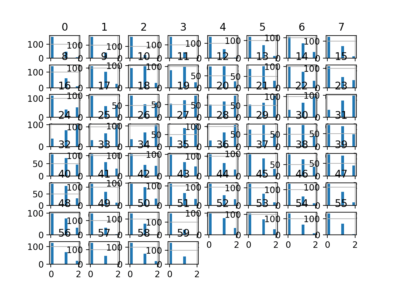
Histogram Plots of K-means Discretization Transformed Input Variables for the Sonar Dataset
Next, let’s evaluate the same KNN model as the previous section, but in this case on a K-means discretization transform of the dataset.
The complete example is listed below.
|
1 2 3 4 5 6 7 8 9 10 11 12 13 14 15 16 17 18 19 20 21 22 23 24 25 26 27 28 29 |
# evaluate knn on the sonar dataset with k-means ordinal discretization transform from numpy import mean from numpy import std from pandas import read_csv from sklearn.model_selection import cross_val_score from sklearn.model_selection import RepeatedStratifiedKFold from sklearn.neighbors import KNeighborsClassifier from sklearn.preprocessing import LabelEncoder from sklearn.preprocessing import KBinsDiscretizer from sklearn.pipeline import Pipeline from matplotlib import pyplot # load dataset url = "https://raw.githubusercontent.com/jbrownlee/Datasets/master/sonar.csv" dataset = read_csv(url, header=None) data = dataset.values # separate into input and output columns X, y = data[:, :-1], data[:, -1] # ensure inputs are floats and output is an integer label X = X.astype('float32') y = LabelEncoder().fit_transform(y.astype('str')) # define the pipeline trans = KBinsDiscretizer(n_bins=3, encode='ordinal', strategy='kmeans') model = KNeighborsClassifier() pipeline = Pipeline(steps=[('t', trans), ('m', model)]) # evaluate the pipeline cv = RepeatedStratifiedKFold(n_splits=10, n_repeats=3, random_state=1) n_scores = cross_val_score(pipeline, X, y, scoring='accuracy', cv=cv, n_jobs=-1, error_score='raise') # report pipeline performance print('Accuracy: %.3f (%.3f)' % (mean(n_scores), std(n_scores))) |
Note: Your results may vary given the stochastic nature of the algorithm or evaluation procedure, or differences in numerical precision. Consider running the example a few times and compare the average outcome.
Running the example, we can see that the K-means discretization transform results in a lift in performance from 79.7 percent accuracy without the transform to about 81.4 percent with the transform, although slightly less than the uniform distribution in the previous section.
|
1 |
Accuracy: 0.814 (0.088) |
Next, let’s take a closer look at the quantile discretization transform.
Quantile Discretization Transform
A quantile discretization transform will attempt to split the observations for each input variable into k groups, where the number of observations assigned to each group is approximately equal.
Unless there are a large number of observations or a complex empirical distribution, the number of bins must be kept small, such as 5-10.
We can apply the quantile discretization transform using the KBinsDiscretizer class and setting the “strategy” argument to “quantile.” We must also set the desired number of bins set via the “n_bins” argument; in this case, we will use 10.
|
1 2 3 4 |
... # perform a quantile discretization transform of the dataset trans = KBinsDiscretizer(n_bins=10, encode='ordinal', strategy='quantile') data = trans.fit_transform(data) |
The example below applies the quantile discretization transform and creates histogram plots of each of the transformed variables.
|
1 2 3 4 5 6 7 8 9 10 11 12 13 14 15 16 17 18 19 |
# visualize a quantile ordinal discretization transform of the sonar dataset from pandas import read_csv from pandas import DataFrame from pandas.plotting import scatter_matrix from sklearn.preprocessing import KBinsDiscretizer from matplotlib import pyplot # load dataset url = "https://raw.githubusercontent.com/jbrownlee/Datasets/master/sonar.csv" dataset = read_csv(url, header=None) # retrieve just the numeric input values data = dataset.values[:, :-1] # perform a quantile discretization transform of the dataset trans = KBinsDiscretizer(n_bins=10, encode='ordinal', strategy='quantile') data = trans.fit_transform(data) # convert the array back to a dataframe dataset = DataFrame(data) # histograms of the variables dataset.hist() pyplot.show() |
Running the example transforms the dataset and plots histograms of each input variable.
We can see that the histograms all show a uniform probability distribution for each input variable, where each of the 10 groups has the same number of observations.
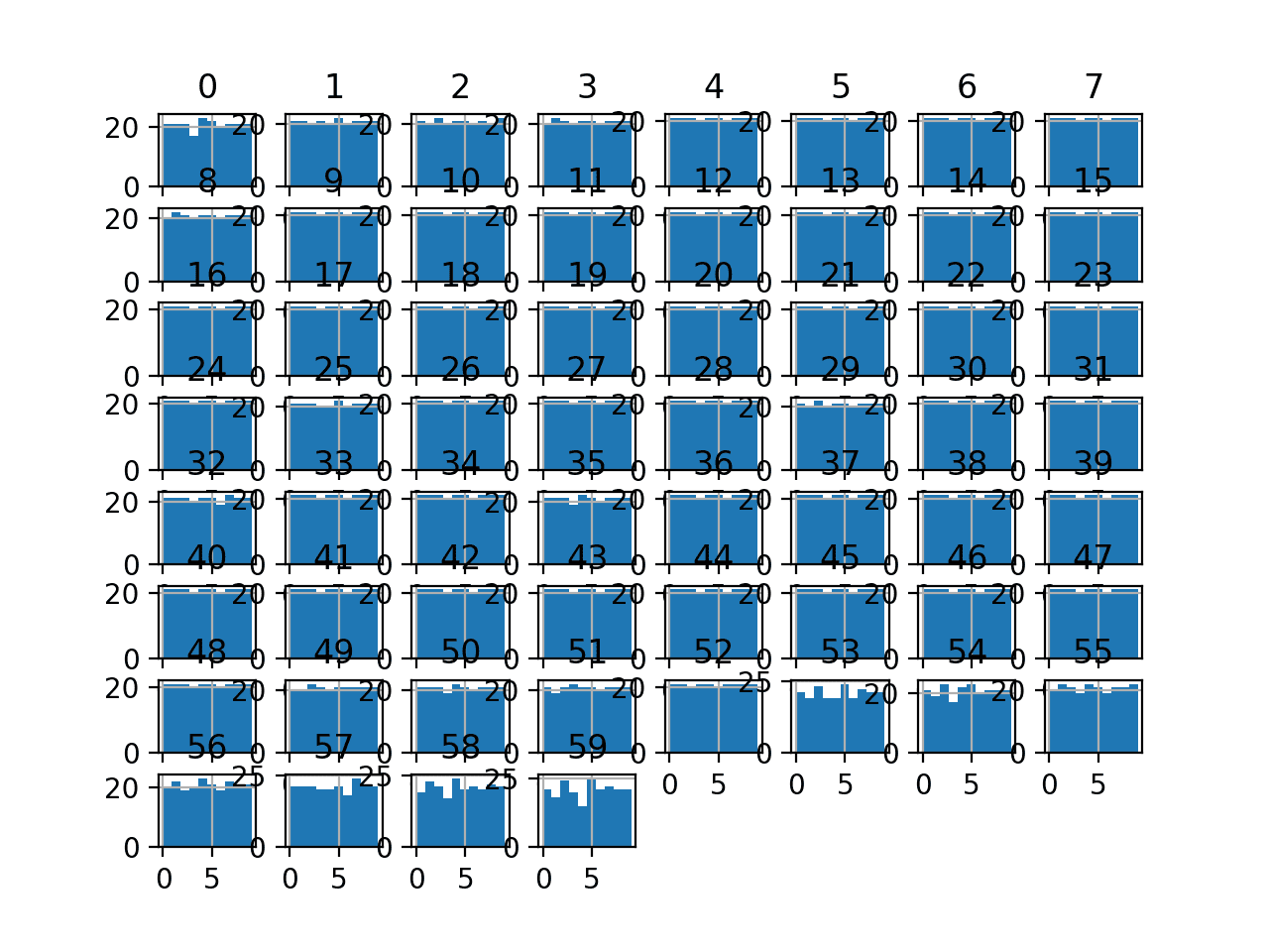
Histogram Plots of Quantile Discretization Transformed Input Variables for the Sonar Dataset
Next, let’s evaluate the same KNN model as the previous section, but in this case, on a quantile discretization transform of the raw dataset.
The complete example is listed below.
|
1 2 3 4 5 6 7 8 9 10 11 12 13 14 15 16 17 18 19 20 21 22 23 24 25 26 27 28 29 |
# evaluate knn on the sonar dataset with quantile ordinal discretization transform from numpy import mean from numpy import std from pandas import read_csv from sklearn.model_selection import cross_val_score from sklearn.model_selection import RepeatedStratifiedKFold from sklearn.neighbors import KNeighborsClassifier from sklearn.preprocessing import LabelEncoder from sklearn.preprocessing import KBinsDiscretizer from sklearn.pipeline import Pipeline from matplotlib import pyplot # load dataset url = "https://raw.githubusercontent.com/jbrownlee/Datasets/master/sonar.csv" dataset = read_csv(url, header=None) data = dataset.values # separate into input and output columns X, y = data[:, :-1], data[:, -1] # ensure inputs are floats and output is an integer label X = X.astype('float32') y = LabelEncoder().fit_transform(y.astype('str')) # define the pipeline trans = KBinsDiscretizer(n_bins=10, encode='ordinal', strategy='quantile') model = KNeighborsClassifier() pipeline = Pipeline(steps=[('t', trans), ('m', model)]) # evaluate the pipeline cv = RepeatedStratifiedKFold(n_splits=10, n_repeats=3, random_state=1) n_scores = cross_val_score(pipeline, X, y, scoring='accuracy', cv=cv, n_jobs=-1, error_score='raise') # report pipeline performance print('Accuracy: %.3f (%.3f)' % (mean(n_scores), std(n_scores))) |
Note: Your results may vary given the stochastic nature of the algorithm or evaluation procedure, or differences in numerical precision. Consider running the example a few times and compare the average outcome.
Running the example, we can see that the uniform transform results in a lift in performance from 79.7 percent accuracy without the transform to about 84.0 percent with the transform, better than the uniform and K-means methods of the previous sections.
|
1 |
Accuracy: 0.840 (0.072) |
We chose the number of bins as an arbitrary number; in this case, 10.
This hyperparameter can be tuned to explore the effect of the resolution of the transform on the resulting skill of the model.
The example below performs this experiment and plots the mean accuracy for different “n_bins” values from two to 10.
|
1 2 3 4 5 6 7 8 9 10 11 12 13 14 15 16 17 18 19 20 21 22 23 24 25 26 27 28 29 30 31 32 33 34 35 36 37 38 39 40 41 42 43 44 45 46 47 48 49 50 51 52 53 54 55 |
# explore number of discrete bins on classification accuracy from numpy import mean from numpy import std from pandas import read_csv from sklearn.model_selection import cross_val_score from sklearn.model_selection import RepeatedStratifiedKFold from sklearn.neighbors import KNeighborsClassifier from sklearn.preprocessing import KBinsDiscretizer from sklearn.preprocessing import LabelEncoder from sklearn.pipeline import Pipeline from matplotlib import pyplot # get the dataset def get_dataset(): # load dataset url = "https://raw.githubusercontent.com/jbrownlee/Datasets/master/sonar.csv" dataset = read_csv(url, header=None) data = dataset.values # separate into input and output columns X, y = data[:, :-1], data[:, -1] # ensure inputs are floats and output is an integer label X = X.astype('float32') y = LabelEncoder().fit_transform(y.astype('str')) return X, y # get a list of models to evaluate def get_models(): models = dict() for i in range(2,11): # define the pipeline trans = KBinsDiscretizer(n_bins=i, encode='ordinal', strategy='quantile') model = KNeighborsClassifier() models[str(i)] = Pipeline(steps=[('t', trans), ('m', model)]) return models # evaluate a give model using cross-validation def evaluate_model(model, X, y): cv = RepeatedStratifiedKFold(n_splits=10, n_repeats=3, random_state=1) scores = cross_val_score(model, X, y, scoring='accuracy', cv=cv, n_jobs=-1, error_score='raise') return scores # get the dataset X, y = get_dataset() # get the models to evaluate models = get_models() # evaluate the models and store results results, names = list(), list() for name, model in models.items(): scores = evaluate_model(model, X, y) results.append(scores) names.append(name) print('>%s %.3f (%.3f)' % (name, mean(scores), std(scores))) # plot model performance for comparison pyplot.boxplot(results, labels=names, showmeans=True) pyplot.show() |
Running the example reports the mean classification accuracy for each value of the “n_bins” argument.
Note: Your results may vary given the stochastic nature of the algorithm or evaluation procedure, or differences in numerical precision. Consider running the example a few times and compare the average outcome.
We can see that surprisingly smaller values resulted in better accuracy, with values such as three achieving an accuracy of about 86.7 percent.
|
1 2 3 4 5 6 7 8 9 |
>2 0.806 (0.080) >3 0.867 (0.070) >4 0.835 (0.083) >5 0.838 (0.070) >6 0.836 (0.071) >7 0.854 (0.071) >8 0.837 (0.077) >9 0.841 (0.069) >10 0.840 (0.072) |
Box and whisker plots are created to summarize the classification accuracy scores for each number of discrete bins on the dataset.
We can see a small bump in accuracy at three bins and the scores drop and remain flat for larger values.
The results highlight that there is likely some benefit in exploring different numbers of discrete bins for the chosen method to see if better performance can be achieved.
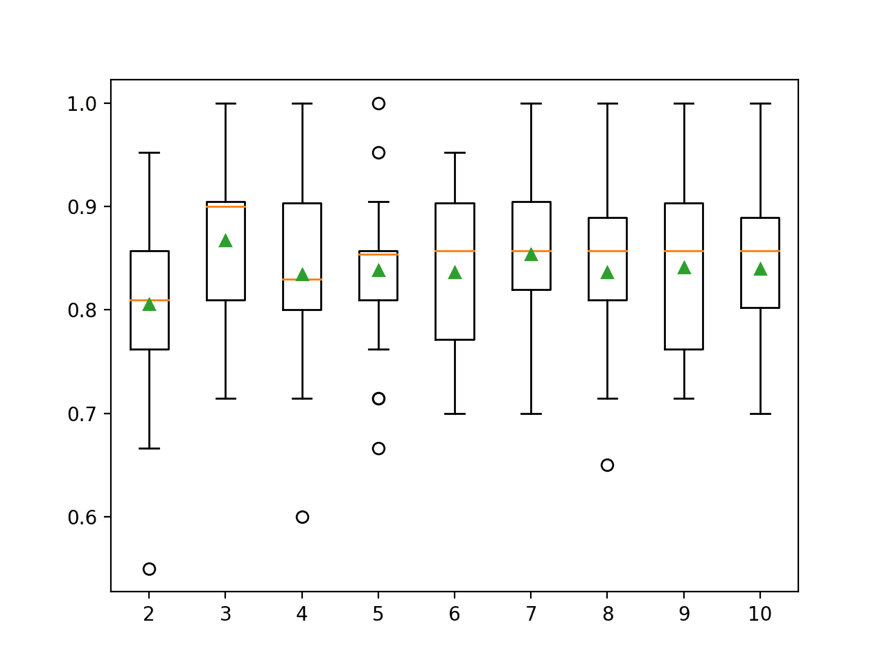
Box Plots of Number of Discrete Bins vs. Classification Accuracy of KNN on the Sonar Dataset
Further Reading
This section provides more resources on the topic if you are looking to go deeper.
Tutorials
- Continuous Probability Distributions for Machine Learning
- How to Transform Target Variables for Regression With Scikit-Learn
Books
- Data Mining: Practical Machine Learning Tools and Techniques, 4th edition, 2016.
- Feature Engineering and Selection, 2019.
Dataset
APIs
Articles
Summary
In this tutorial, you discovered how to use discretization transforms to map numerical values to discrete categories for machine learning.
Specifically, you learned:
- Many machine learning algorithms prefer or perform better when numerical with non-standard probability distributions are made discrete.
- Discretization transforms are a technique for transforming numerical input or output variables to have discrete ordinal labels.
- How to use the KBinsDiscretizer to change the structure and distribution of numeric variables to improve the performance of predictive models.
Do you have any questions?
Ask your questions in the comments below and I will do my best to answer.
Get a Handle on Modern Data Preparation!

Prepare Your Machine Learning Data in Minutes
...with just a few lines of python code
Discover how in my new Ebook:
Data Preparation for Machine Learning
It provides self-study tutorials with full working code on:
Feature Selection, RFE, Data Cleaning, Data Transforms, Scaling, Dimensionality Reduction,
and much more...


Hi Jason,
Thank you for this tutorial.
I would like to use a quantile discretization transform with a tuned number of bins for a random forest model.
Can you please give an example in R using a random forest model?
Do you have any suggestion on this.
Thank you in advance,
Juan
Sorry, I don’t have an example of this in R.
Hi Jason,
thanks for this very cool post. It’s always a pleasure to run the code and see the progress. I understand with this post the need for discretization before running any Machine Learning algorithm.
I compare the above figures with the Neural Network implementation of Sonar dataset with the data preparation “StandarScaler” I reached 87 and 88% or with the Dropout (87,95%). (in your book “Deep Learning With Python”)
My understanding is that we are in the same range of accuracy when running the combination of { k-nearest neighbor algorithm and repeated stratified k-fold stratified + discretization} or {Neural Network model + StandarScaler + Dropout}.
So my question: do you have a recommendation between the two types of Machine Learning Algorithms? (between the Instance Based kNN and the Neural Network MLP)
Thanks,
Kind regards
Dominique
Thanks.
No, always test a suite of algorithms and data prep methods, whole modeling pipelines, in order to discover what works best for a dataset.
Hello Jason,
Thankyou very much for sharing your knowledge. I read about an algorithm that can help us discretize the target variable. I would really like to hear your thoughts on this.
https://www.ncbi.nlm.nih.gov/pmc/articles/PMC5148156/
You’re welcome.
Sorry, I am not familiar with that work.
Hello Jason,
Thankyou. I have a. question, when doing the quantile discretization transform, should we do that in the whole dataset?
or should we split train – test and do it only in train set??
The transform must be fit on the training set and applied to the train and test sets.
You can do this automatically with a pipeline when using cross validation.
Thank you so much for giving the information. The discretization transform is explained very nicely. I am really thank you for for sharing everything with an example.
You’re welcome.
This is a really illustrative tutorial! I would additionally like to know if there is any method to quantify the information loss when performing discretization transformation.
Thanks!
Good question, I have not done this myself. Perhaps check the literature for a common approach to measuring the change in information, or perhaps start with something like a divergence measure:
https://machinelearningmastery.com/divergence-between-probability-distributions/
This is very interesting Jason. Thanks for sharing.
After doing the discretization, how can we see the different bins? The thresholds?
Thanks.
Great question! See the “n_bins_” and “bin_edges_” attributes on your KBinsDiscretizer instance.
More details here:
https://scikit-learn.org/stable/modules/generated/sklearn.preprocessing.KBinsDiscretizer.html
Hi Jason,
Many thanks for your nice sharing of the unsupervised discretization methods! The code examples including the pipeline is very helpful. With the pipeline, data leakage can be avoided.
Here I have one question. What do you think of supervised discretization method, such as DecisionTreeDiscretiser.
I’m working on the Kaggle competition of Titanic and planning on discretizing age and fare variables.
Try it and see if it improves performance on your project.
Why do you apply for all columns same strategy? How to proceed when data contains numerical, categorical and ordinal columns?
Just as a demonstration.
Hi Jason,
I have a simple question,
How we can determine the number of bins?
i.e is there any numerical method to choose how many “k discrete bins” must be used?
No, grid search a range of values and use a configration that works well or best for your dataset and chosen model.
Thank you
You’re welcome.
Hi Jason
Let’s say we have “age” and “income” as feature, we want to group for example:
age 1-12 : group age A
age 13-30 : group age B
age 31-40 : group age C, etc
income 1-100 : group Income A
income 101-150 : group Income B
income 151-250 : group Income C,etc
Each group maybe has different range, is there any way, to “search” the range of Age and Income for each group, that when is used to Y target(maybe sentiment analysis), this range of age and income in each group can be optimal to the Y target?
Thanks
Mike
Probably you want to do some heuristic search to find the optimal. Simulated annealing, for example.
Hello, thank you for this tutorial. I had a question, as KNN uses the Euclidean distance technique, how can we use the ordinal variable in this algorithm?
Hi Mehdi…Thank you for your feedback! Please elaborate on your goals with KNN and the ordinal variable so that we may better assist you.