
Autoencoder is a type of neural network that can be used to learn a compressed representation of raw data.
An autoencoder is composed of encoder and a decoder sub-models. The encoder compresses the input and the decoder attempts to recreate the input from the compressed version provided by the encoder. After training, the encoder model is saved and the decoder is discarded.
The encoder can then be used as a data preparation technique to perform feature extraction on raw data that can be used to train a different machine learning model.
In this tutorial, you will discover how to develop and evaluate an autoencoder for regression predictive
After completing this tutorial, you will know:
- An autoencoder is a neural network model that can be used to learn a compressed representation of raw data.
- How to train an autoencoder model on a training dataset and save just the encoder part of the model.
- How to use the encoder as a data preparation step when training a machine learning model.
Let’s get started.

Autoencoder Feature Extraction for Regression
Photo by Simon Matzinger, some rights reserved.
Tutorial Overview
This tutorial is divided into three parts; they are:
- Autoencoders for Feature Extraction
- Autoencoder for Regression
- Autoencoder as Data Preparation
Autoencoders for Feature Extraction
An autoencoder is a neural network model that seeks to learn a compressed representation of an input.
An autoencoder is a neural network that is trained to attempt to copy its input to its output.
— Page 502, Deep Learning, 2016.
They are an unsupervised learning method, although technically, they are trained using supervised learning methods, referred to as self-supervised. They are typically trained as part of a broader model that attempts to recreate the input.
For example:
- X = model.predict(X)
The design of the autoencoder model purposefully makes this challenging by restricting the architecture to a bottleneck at the midpoint of the model, from which the reconstruction of the input data is performed.
There are many types of autoencoders, and their use varies, but perhaps the more common use is as a learned or automatic feature extraction model.
In this case, once the model is fit, the reconstruction aspect of the model can be discarded and the model up to the point of the bottleneck can be used. The output of the model at the bottleneck is a fixed length vector that provides a compressed representation of the input data.
Usually they are restricted in ways that allow them to copy only approximately, and to copy only input that resembles the training data. Because the model is forced to prioritize which aspects of the input should be copied, it often learns useful properties of the data.
— Page 502, Deep Learning, 2016.
Input data from the domain can then be provided to the model and the output of the model at the bottleneck can be used as a feature vector in a supervised learning model, for visualization, or more generally for dimensionality reduction.
Next, let’s explore how we might develop an autoencoder for feature extraction on a regression predictive modeling problem.
Autoencoder for Regression
In this section, we will develop an autoencoder to learn a compressed representation of the input features for a regression predictive modeling problem.
First, let’s define a regression predictive modeling problem.
We will use the make_regression() scikit-learn function to define a synthetic regression task with 100 input features (columns) and 1,000 examples (rows). Importantly, we will define the problem in such a way that most of the input variables are redundant (90 of the 100 or 90 percent), allowing the autoencoder later to learn a useful compressed representation.
The example below defines the dataset and summarizes its shape.
|
1 2 3 4 5 6 |
# synthetic regression dataset from sklearn.datasets import make_regression # define dataset X, y = make_regression(n_samples=1000, n_features=100, n_informative=10, noise=0.1, random_state=1) # summarize the dataset print(X.shape, y.shape) |
Running the example defines the dataset and prints the shape of the arrays, confirming the number of rows and columns.
|
1 |
(1000, 100) (1000,) |
Next, we will develop a Multilayer Perceptron (MLP) autoencoder model.
The model will take all of the input columns, then output the same values. It will learn to recreate the input pattern exactly.
The autoencoder consists of two parts: the encoder and the decoder. The encoder learns how to interpret the input and compress it to an internal representation defined by the bottleneck layer. The decoder takes the output of the encoder (the bottleneck layer) and attempts to recreate the input.
Once the autoencoder is trained, the decode is discarded and we only keep the encoder and use it to compress examples of input to vectors output by the bottleneck layer.
In this first autoencoder, we won’t compress the input at all and will use a bottleneck layer the same size as the input. This should be an easy problem that the model will learn nearly perfectly and is intended to confirm our model is implemented correctly.
We will define the model using the functional API. If this is new to you, I recommend this tutorial:
Prior to defining and fitting the model, we will split the data into train and test sets and scale the input data by normalizing the values to the range 0-1, a good practice with MLPs.
|
1 2 3 4 5 6 7 8 |
... # split into train test sets X_train, X_test, y_train, y_test = train_test_split(X, y, test_size=0.33, random_state=1) # scale data t = MinMaxScaler() t.fit(X_train) X_train = t.transform(X_train) X_test = t.transform(X_test) |
We will define the encoder to have one hidden layer with the same number of nodes as there are in the input data with batch normalization and ReLU activation.
This is followed by a bottleneck layer with the same number of nodes as columns in the input data, e.g. no compression.
|
1 2 3 4 5 6 7 8 9 |
... # define encoder visible = Input(shape=(n_inputs,)) e = Dense(n_inputs*2)(visible) e = BatchNormalization()(e) e = ReLU()(e) # define bottleneck n_bottleneck = n_inputs bottleneck = Dense(n_bottleneck)(e) |
The decoder will be defined with the same structure.
It will have one hidden layer with batch normalization and ReLU activation. The output layer will have the same number of nodes as there are columns in the input data and will use a linear activation function to output numeric values.
|
1 2 3 4 5 6 7 8 9 10 11 |
... # define decoder d = Dense(n_inputs*2)(bottleneck) d = BatchNormalization()(d) d = ReLU()(d) # output layer output = Dense(n_inputs, activation='linear')(d) # define autoencoder model model = Model(inputs=visible, outputs=output) # compile autoencoder model model.compile(optimizer='adam', loss='mse') |
The model will be fit using the efficient Adam version of stochastic gradient descent and minimizes the mean squared error, given that reconstruction is a type of multi-output regression problem.
|
1 2 3 |
... # compile autoencoder model model.compile(optimizer='adam', loss='mse') |
We can plot the layers in the autoencoder model to get a feeling for how the data flows through the model.
|
1 2 3 |
... # plot the autoencoder plot_model(model, 'autoencoder.png', show_shapes=True) |
The image below shows a plot of the autoencoder.
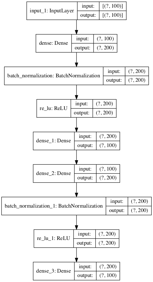
Plot of the Autoencoder Model for Regression
Next, we can train the model to reproduce the input and keep track of the performance of the model on the holdout test set. The model is trained for 400 epochs and a batch size of 16 examples.
|
1 2 3 |
... # fit the autoencoder model to reconstruct input history = model.fit(X_train, X_train, epochs=400, batch_size=16, verbose=2, validation_data=(X_test,X_test)) |
After training, we can plot the learning curves for the train and test sets to confirm the model learned the reconstruction problem well.
|
1 2 3 4 5 6 |
... # plot loss pyplot.plot(history.history['loss'], label='train') pyplot.plot(history.history['val_loss'], label='test') pyplot.legend() pyplot.show() |
Finally, we can save the encoder model for use later, if desired.
|
1 2 3 4 5 6 |
... # define an encoder model (without the decoder) encoder = Model(inputs=visible, outputs=bottleneck) plot_model(encoder, 'encoder.png', show_shapes=True) # save the encoder to file encoder.save('encoder.h5') |
As part of saving the encoder, we will also plot the model to get a feeling for the shape of the output of the bottleneck layer, e.g. a 100-element vector.
An example of this plot is provided below.
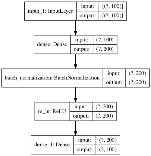
Plot of Encoder Model for Regression With No Compression
Tying this all together, the complete example of an autoencoder for reconstructing the input data for a regression dataset without any compression in the bottleneck layer is listed below.
|
1 2 3 4 5 6 7 8 9 10 11 12 13 14 15 16 17 18 19 20 21 22 23 24 25 26 27 28 29 30 31 32 33 34 35 36 37 38 39 40 41 42 43 44 45 46 47 48 49 50 51 52 53 54 |
# train autoencoder for regression with no compression in the bottleneck layer from sklearn.datasets import make_regression from sklearn.preprocessing import MinMaxScaler from sklearn.model_selection import train_test_split from tensorflow.keras.models import Model from tensorflow.keras.layers import Input from tensorflow.keras.layers import Dense from tensorflow.keras.layers import ReLU from tensorflow.keras.layers import BatchNormalization from tensorflow.keras.utils import plot_model from matplotlib import pyplot # define dataset X, y = make_regression(n_samples=1000, n_features=100, n_informative=10, noise=0.1, random_state=1) # number of input columns n_inputs = X.shape[1] # split into train test sets X_train, X_test, y_train, y_test = train_test_split(X, y, test_size=0.33, random_state=1) # scale data t = MinMaxScaler() t.fit(X_train) X_train = t.transform(X_train) X_test = t.transform(X_test) # define encoder visible = Input(shape=(n_inputs,)) e = Dense(n_inputs*2)(visible) e = BatchNormalization()(e) e = ReLU()(e) # define bottleneck n_bottleneck = n_inputs bottleneck = Dense(n_bottleneck)(e) # define decoder d = Dense(n_inputs*2)(bottleneck) d = BatchNormalization()(d) d = ReLU()(d) # output layer output = Dense(n_inputs, activation='linear')(d) # define autoencoder model model = Model(inputs=visible, outputs=output) # compile autoencoder model model.compile(optimizer='adam', loss='mse') # plot the autoencoder plot_model(model, 'autoencoder.png', show_shapes=True) # fit the autoencoder model to reconstruct input history = model.fit(X_train, X_train, epochs=400, batch_size=16, verbose=2, validation_data=(X_test,X_test)) # plot loss pyplot.plot(history.history['loss'], label='train') pyplot.plot(history.history['val_loss'], label='test') pyplot.legend() pyplot.show() # define an encoder model (without the decoder) encoder = Model(inputs=visible, outputs=bottleneck) plot_model(encoder, 'encoder.png', show_shapes=True) # save the encoder to file encoder.save('encoder.h5') |
Running the example fits the model and reports loss on the train and test sets along the way.
Note: if you have problems creating the plots of the model, you can comment out the import and call the plot_model() function.
Note: Your results may vary given the stochastic nature of the algorithm or evaluation procedure, or differences in numerical precision. Consider running the example a few times and compare the average outcome.
In this case, we see that loss gets low but does not go to zero (as we might have expected) with no compression in the bottleneck layer. Perhaps further tuning the model architecture or learning hyperparameters is required.
|
1 2 3 4 5 6 7 8 9 10 11 12 13 14 15 16 17 |
... Epoch 393/400 42/42 - 0s - loss: 0.0025 - val_loss: 0.0024 Epoch 394/400 42/42 - 0s - loss: 0.0025 - val_loss: 0.0021 Epoch 395/400 42/42 - 0s - loss: 0.0023 - val_loss: 0.0021 Epoch 396/400 42/42 - 0s - loss: 0.0025 - val_loss: 0.0023 Epoch 397/400 42/42 - 0s - loss: 0.0024 - val_loss: 0.0022 Epoch 398/400 42/42 - 0s - loss: 0.0025 - val_loss: 0.0021 Epoch 399/400 42/42 - 0s - loss: 0.0026 - val_loss: 0.0022 Epoch 400/400 42/42 - 0s - loss: 0.0025 - val_loss: 0.0024 |
A plot of the learning curves is created showing that the model achieves a good fit in reconstructing the input, which holds steady throughout training, not overfitting.
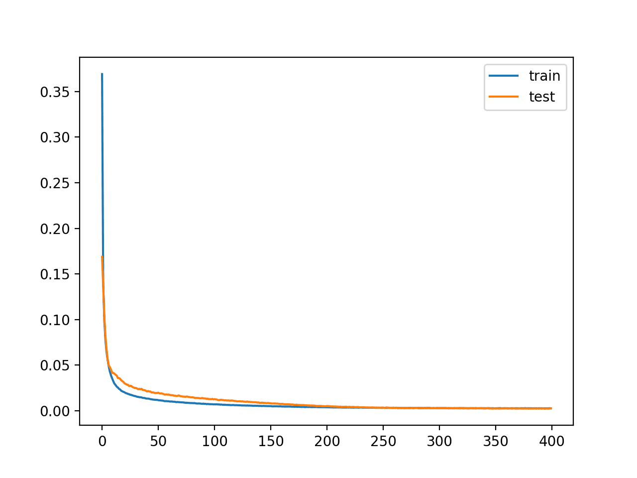
Learning Curves of Training the Autoencoder Model for Regression Without Compression
So far, so good. We know how to develop an autoencoder without compression.
The trained encoder is saved to the file “encoder.h5” that we can load and use later.
Next, let’s explore how we might use the trained encoder model.
Autoencoder as Data Preparation
In this section, we will use the trained encoder model from the autoencoder model to compress input data and train a different predictive model.
First, let’s establish a baseline in performance on this problem. This is important as if the performance of a model is not improved by the compressed encoding, then the compressed encoding does not add value to the project and should not be used.
We can train a support vector regression (SVR) model on the training dataset directly and evaluate the performance of the model on the holdout test set.
As is good practice, we will scale both the input variables and target variable prior to fitting and evaluating the model.
The complete example is listed below.
|
1 2 3 4 5 6 7 8 9 10 11 12 13 14 15 16 17 18 19 20 21 22 23 24 25 26 27 28 29 30 31 32 33 34 35 36 |
# baseline in performance with support vector regression model from sklearn.datasets import make_regression from sklearn.preprocessing import MinMaxScaler from sklearn.model_selection import train_test_split from sklearn.svm import SVR from sklearn.metrics import mean_absolute_error # define dataset X, y = make_regression(n_samples=1000, n_features=100, n_informative=10, noise=0.1, random_state=1) # split into train test sets X_train, X_test, y_train, y_test = train_test_split(X, y, test_size=0.33, random_state=1) # reshape target variables so that we can transform them y_train = y_train.reshape((len(y_train), 1)) y_test = y_test.reshape((len(y_test), 1)) # scale input data trans_in = MinMaxScaler() trans_in.fit(X_train) X_train = trans_in.transform(X_train) X_test = trans_in.transform(X_test) # scale output data trans_out = MinMaxScaler() trans_out.fit(y_train) y_train = trans_out.transform(y_train) y_test = trans_out.transform(y_test) # define model model = SVR() # fit model on the training dataset model.fit(X_train, y_train) # make prediction on test set yhat = model.predict(X_test) # invert transforms so we can calculate errors yhat = yhat.reshape((len(yhat), 1)) yhat = trans_out.inverse_transform(yhat) y_test = trans_out.inverse_transform(y_test) # calculate error score = mean_absolute_error(y_test, yhat) print(score) |
Running the example fits an SVR model on the training dataset and evaluates it on the test set.
Note: Your results may vary given the stochastic nature of the algorithm or evaluation procedure, or differences in numerical precision. Consider running the example a few times and compare the average outcome.
In this case, we can see that the model achieves a mean absolute error (MAE) of about 89.
We would hope and expect that a SVR model fit on an encoded version of the input to achieve lower error for the encoding to be considered useful.
|
1 |
89.51082036130629 |
We can update the example to first encode the data using the encoder model trained in the previous section.
First, we can load the trained encoder model from the file.
|
1 2 3 |
... # load the model from file encoder = load_model('encoder.h5') |
We can then use the encoder to transform the raw input data (e.g. 100 columns) into bottleneck vectors (e.g. 100 element vectors).
This process can be applied to the train and test datasets.
|
1 2 3 4 5 |
... # encode the train data X_train_encode = encoder.predict(X_train) # encode the test data X_test_encode = encoder.predict(X_test) |
We can then use this encoded data to train and evaluate the SVR model, as before.
|
1 2 3 4 5 6 7 |
... # define model model = SVR() # fit model on the training dataset model.fit(X_train_encode, y_train) # make prediction on test set yhat = model.predict(X_test_encode) |
Tying this together, the complete example is listed below.
|
1 2 3 4 5 6 7 8 9 10 11 12 13 14 15 16 17 18 19 20 21 22 23 24 25 26 27 28 29 30 31 32 33 34 35 36 37 38 39 40 41 42 43 |
# support vector regression performance with encoded input from sklearn.datasets import make_regression from sklearn.preprocessing import MinMaxScaler from sklearn.model_selection import train_test_split from sklearn.svm import SVR from sklearn.metrics import mean_absolute_error from tensorflow.keras.models import load_model # define dataset X, y = make_regression(n_samples=1000, n_features=100, n_informative=10, noise=0.1, random_state=1) # split into train test sets X_train, X_test, y_train, y_test = train_test_split(X, y, test_size=0.33, random_state=1) # reshape target variables so that we can transform them y_train = y_train.reshape((len(y_train), 1)) y_test = y_test.reshape((len(y_test), 1)) # scale input data trans_in = MinMaxScaler() trans_in.fit(X_train) X_train = trans_in.transform(X_train) X_test = trans_in.transform(X_test) # scale output data trans_out = MinMaxScaler() trans_out.fit(y_train) y_train = trans_out.transform(y_train) y_test = trans_out.transform(y_test) # load the model from file encoder = load_model('encoder.h5') # encode the train data X_train_encode = encoder.predict(X_train) # encode the test data X_test_encode = encoder.predict(X_test) # define model model = SVR() # fit model on the training dataset model.fit(X_train_encode, y_train) # make prediction on test set yhat = model.predict(X_test_encode) # invert transforms so we can calculate errors yhat = yhat.reshape((len(yhat), 1)) yhat = trans_out.inverse_transform(yhat) y_test = trans_out.inverse_transform(y_test) # calculate error score = mean_absolute_error(y_test, yhat) print(score) |
Running the example first encodes the dataset using the encoder, then fits an SVR model on the training dataset and evaluates it on the test set.
Note: Your results may vary given the stochastic nature of the algorithm or evaluation procedure, or differences in numerical precision. Consider running the example a few times and compare the average outcome.
In this case, we can see that the model achieves a MAE of about 69.
This is a better MAE than the same model evaluated on the raw dataset, suggesting that the encoding is helpful for our chosen model and test harness.
|
1 |
69.45890939600503 |
Further Reading
This section provides more resources on the topic if you are looking to go deeper.
Tutorials
- A Gentle Introduction to LSTM Autoencoders
- How to Use the Keras Functional API for Deep Learning
- TensorFlow 2 Tutorial: Get Started in Deep Learning With tf.keras
Books
- Deep Learning, 2016.
APIs
Articles
Summary
In this tutorial, you discovered how to develop and evaluate an autoencoder for regression predictive modeling.
Specifically, you learned:
- An autoencoder is a neural network model that can be used to learn a compressed representation of raw data.
- How to train an autoencoder model on a training dataset and save just the encoder part of the model.
- How to use the encoder as a data preparation step when training a machine learning model.
Do you have any questions?
Ask your questions in the comments below and I will do my best to answer.


 for Feature Selection in Python")
Hi Jason, I have two questions:
1. Given that we set the compression size to 100 (no compression), we should in theory achieve a reconstruction error of zero. Why is this not the case?
3. Considering that we are not compressing, how is it possible that we achieve a smaller MAE?
To extract salient features, we should set compression size (size of bottleneck) to a number smaller than 100, right?
Best,
Gabriele
Some ideas: the problem may be too hard to learn perfectly for this model, more tuning of the architecture and learning hyperparametres is required, etc.
Better representation results in better learning, the same reason we use data transforms on raw data, like scaling or power transforms.
Thanks Jason! And thank you for your blog posting.
You’re welcome.
Thank you for this tutorial. I believe that before you save the encoder to encoder.h5 file, you need to compile it.
You can if you like, it will not impact performance as we will not train it – and compile() is only relevant for training model.
If you don’t compile it, I get a warning and the results are very different.
You can safely ignore that warning.
Thanks Jason,
This tutorial came on time.
If I have two different sets of inputs. The first has the shape n*m , the second has n*1
I want to use both sets as inputs.
Can you give me a clue what is the proper way to build a model using these two sets, with the first one being encoded using an autoencoder, please?
More clarification: the input shape for the autoencoder is different from the input shape of the prediction model.
Yes, this example uses a different shape input for the autoencoder and the predictive model:
https://machinelearningmastery.com/autoencoder-for-classification/
Perhaps you can use a separate input for each model, this may help:
https://machinelearningmastery.com/keras-functional-api-deep-learning/
Hi Jason,
I noticed, that on artificial regression datasets like sklearn.datasets.make_regression you have used in this tutorial, learning curves often do not show any sign of overfitting.
For example, recently I’ve done some experiments with training neural networks on make_friedman group of dataset generators from the same sklearn.datasets, and was unable to force my network to overfit on them whatever I do.
Do you have an idea what’s wrong here?
Perhaps use less noise in the dataset.
Hi Jason,
Thank you for your tutorials, it is a big contribution to “machine learning democratization” for an open educational world !
As I did on your analogue autoencoder tutorial for classification, I performed several variants to your baseline code, in order to experiment with autoencoder statistical sensitivity vs different regression models, different grade of feature compression and for KFold (different groups of model training/test), so :
– I applied comparison analysis for 5 models (linearRegression, SVR, RandomForestRegressor, ExtraTreesRegressor, XGBRegressor)
– I applied comparison analysis for different grade of compression (none -raw inputs without autoencoding-, 1, 1/2)
– I applied statistical analysis for different training/test dataset groups (KFold with repetition)
so I used “cross_val_score” function of Sklearn and in order to apply MAE scoring within it, I use “make_score” wrapper of Sklearn.
My conclusions:
– similar to the one provides on your equivalent classification tutorial. The results are more sensitive to the learning model chosen than apply (o not) autoencoder.
– In my case I got the best resuts with LinearRegression model (very optimal), but also I checkout that using SVR model applying autoencoder is best than do not do it. But in the rest of models sometines results are better without applying autoencoder
– I also changed your autoencoder model, and apply the same one used on classification, where you have some kind of two blocks of encoder/decoder…the results are a little bit worse than using your simple encoder/decoder of this tutorial.
as a summary, as you said, all of these techniques are Heuristic, so we have to try many tools and measure the results
thank you Jason !
Thank you for your kind words.
Very impressive experiments!
Yes, I found regression more challenging than the classification example to prepare. Likely because of the chosen synthetic dataset. A linear regression can solve the synthetic dataset optimally, I try to avoid it when using this dataset.
I tried to run the same code but got this error. Please tell me what mistake i am doing.
FailedPreconditionError: Could not find variable dense_30/kernel. This could mean that the variable has been deleted. In TF1, it can also mean the variable is uninitialized. Debug info: container=localhost, status=Not found: Resource localhost/dense_30/kernel/class tensorflow::Var does not exist.
[[{{node dense_30/MatMul/ReadVariableOp}}]]
I cannot tell. May be you need to simplify your code and debug to see how this error occurred.
Hi,
This is a very useful tutorial! However, mainly due to my lack of coding experience, I have some doubts, and I would be grateful to you if you could help me!
1) In this example, you have split one single dataset into two parts training (0.67) and test (0.33), right? However, when I have the training and test previously defined into two different data files (e.g., “train.csv” and “test.csv”), how can I handle this?
2) Both train and test files are composed of 26 columns (train=20631 rows and test=13096 rows), being:
C1 = engine number (100 different engines)
C2 = time, in cycles (target)
C3 to C5 = operational settings (constant to all the 100 engines)
C6 to C26 = sensor measurements – 21 columns
Should I keep all the columns? Or can I exclude, for instance, C1 and C3 to C5, since C1 is not informative and C3 to C5 are constant throughout the observations?
3) What is the right way of setting the parameters: n_samples = (rows of “train.csv” + rows of “test.csv” ?); n_features= (21?); n_informative=(what would be?)
I really sorry for the extensive number of questions, but I have the feeling that this place has been the only one where I can find useful and clear information in this field!
Many thanks for considering my request.
You have to first clarify to yourself the target of your research.
Do you want to predict C2 based on C6 to C26? Then that’s all you need. After all, can a constant value affect your prediction?
More specifically, and assuming you are regressing against column C2:
1) You either use the train and test as provided to you, or you can merge and shuffle them to create a master database, and from there on use the code by Jason (which also shuffles, by the way).
If you meant ‘how to do it in practice’, i.e. how to use the data given to you… well, one fast approach would be to load the data with pandas.read_csv and then convert them to numpy. One file will be your X_train and the other will be the X_test. Of course you have to put column C2 in the relevant y_train and y_test. Check pandas.read_csv documentation to see how to do it quickly and efficiently (hint: you can select which columns to read).
2) Answered above.
3) Those parameters only refer to sklearn.datasets.make_regression.
This is a function used to create artificial data.
You will be not using it, so you don’t care to set n_informative (actually, the idea of your analysis should be _exactly_ to figure out which features are informative!).
In case you are curious, the equivalent would be that n_samples is the shape of your X (np.shape(X)[0]), whatever you decide to use (the data as they are given you, or the merged and resampled data). But again, you won’t need it.
Thank you for your good training.
I have a question. Shouldn’t the size of the hidden layers and the size of the bottleneck be smaller than the size of the input layer (less than 100)?
Hi barad…The following discussion may be of interest to you:
https://www.researchgate.net/post/How-to-configure-the-size-of-hidden-nodes-code-in-an-autoencoder
How do i get the decoder?
Hi Rogerio…The following resource may be of interest:
https://machinelearningmastery.com/implementing-the-transformer-decoder-from-scratch-in-tensorflow-and-keras/
thank alot for your generosity in free learning. i have a question. you one time inside autoencoder change scale of data and used MinMAx() and output of that was used inside SVR, and again another time inside SVR model you used MinMAX()?
twice scaling don’t have significant effect on result?
Hi vahid…There is no issue.
Thank you for providing this helpful tutorial. I’ve recently started studying and practicing with autoencoders, so I hope my question isn’t too basic. If one chooses to use compression, designing the bottleneck layer with a dimension smaller than the input layer, is it necessary to export the decoder as well? Or can the regression model be directly applied to the representation in the latent space?
Thank you!
Hi gallog-hash…You are very welcome! Your understanding is correct, the regression model can be directly applied to the representation in the latent space. Let us know what you build with your model!