Time Series Forecast Case Study with Python: Monthly Armed Robberies in Boston

Time series forecasting is a process, and the only way to get good forecasts is to practice this process.

In this tutorial, you will discover how to forecast the number of monthly armed robberies in Boston with Python.

Working through this tutorial will provide you with a framework for the steps and the tools for working through your own time series forecasting problems.

After completing this tutorial, you will know:

• How to check your Python environment and carefully define a time series forecasting problem.
• How to create a test harness for evaluating models, develop a baseline forecast, and better understand your problem with the tools of time series analysis.
• How to develop an autoregressive integrated moving average model, save it to file, and later load it to make predictions for new time steps.

Kick-start your project with my new book Time Series Forecasting With Python, including step-by-step tutorials and the Python source code files for all examples.

Let’s get started.

• Updated Jul/2018: Fixed a typo in the preparation of the ACF/PACF plots (thanks Patrick Wolf).
• Updated Apr/2019: Updated the link to dataset.
• Updated Aug/2019: Updated data loading to use new API.
• Updated Feb/2020: Updated to_csv() to remove warnings.
• Updated Dec/2020: Updated modeling for changes to the API.

Time Series Forecast Case Study with Python – Monthly Armed Robberies in Boston
Photo by Tim Sackton, some rights reserved.

Overview

In this tutorial, we will work through a time series forecasting project from end-to-end, from downloading the dataset and defining the problem to training a final model and making predictions.

This project is not exhaustive, but shows how you can get good results quickly by working through a time series forecasting problem systematically.

The steps of this project that we will work through are as follows:

1. Environment.
2. Problem Description.
3. Test Harness.
4. Persistence.
5. Data Analysis.
6. ARIMA Models
7. Model Validation

This will provide a template for working through a time series prediction problem that you can use on your own dataset.

1. Environment

This tutorial assumes an installed and working SciPy environment and dependencies, including:

• SciPy
• NumPy
• Matplotlib
• Pandas
• scikit-learn
• statsmodels

I used Python 2.7. Are you on Python 3? let me know how you go in the comments.

This script will help you check your installed versions of these libraries.

The results on my workstation used to write this tutorial are as follows:

2. Problem Description

The problem is to predict the number of monthly armed robberies in Boston, USA.

The dataset provides the number of monthly armed robberies in Boston from January 1966 to October 1975, or just under 10 years of data.

The values are a count and there are 118 observations.

The dataset is credited to McCleary & Hay (1980).

• Download the dataset.

Download the dataset as a CSV file and place it in your current working directory with the filename “robberies.csv“.

3. Test Harness

We must develop a test harness to investigate the data and evaluate candidate models.

This involves two steps:

1. Defining a Validation Dataset.
2. Developing a Method for Model Evaluation.

3.1 Validation Dataset

The dataset is not current. This means that we cannot easily collect updated data to validate the model.

Therefore we will pretend that it is October 1974 and withhold the last one year of data from analysis and model selection.

This final year of data will be used to validate the final model.

The code below will load the dataset as a Pandas Series and split into two, one for model development (dataset.csv) and the other for validation (validation.csv).

Running the example creates two files and prints the number of observations in each.

The specific contents of these files are:

• dataset.csv: Observations from January 1966 to October 1974 (106 observations)
• validation.csv: Observations from November 1974 to October 1975 (12 observations)

The validation dataset is 10% of the original dataset.

Note that the saved datasets do not have a header line, therefore we do not need to cater to this when working with these files later.

3.2. Model Evaluation

Model evaluation will only be performed on the data in dataset.csv prepared in the previous section.

Model evaluation involves two elements:

1. Performance Measure.
2. Test Strategy.

3.2.1 Performance Measure

The observations are a count of robberies.

We will evaluate the performance of predictions using the root mean squared error (RMSE). This will give more weight to predictions that are grossly wrong and will have the same units as the original data.

Any transforms to the data must be reversed before the RMSE is calculated and reported to make the performance between different methods directly comparable.

We can calculate the RMSE using the helper function from the scikit-learn library mean_squared_error() that calculates the mean squared error between a list of expected values (the test set) and the list of predictions. We can then take the square root of this value to give us an RMSE score.

For example:

3.2.2 Test Strategy

Candidate models will be evaluated using walk-forward validation.

This is because a rolling-forecast type model is required from the problem definition. This is where one-step forecasts are needed given all available data.

The walk-forward validation will work as follows:

• The first 50% of the dataset will be held back to train the model.
• The remaining 50% of the dataset will be iterated and test the model.
• For each step in the test dataset:
  • A model will be trained.
  • A one-step prediction made and the prediction stored for later evaluation.
  • The actual observation from the test dataset will be added to the training dataset for the next iteration.
• The predictions made during the iteration of the test dataset will be evaluated and an RMSE score reported.

Given the small size of the data, we will allow a model to be re-trained given all available data prior to each prediction.

We can write the code for the test harness using simple NumPy and Python code.

Firstly, we can split the dataset into train and test sets directly. We’re careful to always convert a loaded dataset to float32 in case the loaded data still has some String or Integer data types.

Next, we can iterate over the time steps in the test dataset. The train dataset is stored in a Python list as we need to easily append a new observation each iteration and Numpy array concatenation feels like overkill.

The prediction made by the model is called yhat for convention, as the outcome or observation is referred to as y and yhat (a ‘y‘ with a mark above) is the mathematical notation for the prediction of the y variable.

The prediction and observation are printed each observation for a sanity check prediction in case there are issues with the model.

4. Persistence

The first step before getting bogged down in data analysis and modeling is to establish a baseline of performance.

This will provide both a template for evaluating models using the proposed test harness and a performance measure by which all more elaborate predictive models can be compared.

The baseline prediction for time series forecasting is called the naive forecast, or persistence.

This is where the observation from the previous time step is used as the prediction for the observation at the next time step.

We can plug this directly into the test harness defined in the previous section.

The complete code listing is provided below.

Running the test harness prints the prediction and observation for each iteration of the test dataset.

The example ends by printing the RMSE for the model.

In this case, we can see that the persistence model achieved an RMSE of 51.844. This means that on average, the model was wrong by about 51 robberies for each prediction made.

We now have a baseline prediction method and performance; now we can start digging into our data.

5. Data Analysis

We can use summary statistics and plots of the data to quickly learn more about the structure of the prediction problem.

In this section, we will look at the data from four perspectives:

1. Summary Statistics.
2. Line Plot.
3. Density Plots.
4. Box and Whisker Plot.

5.1 Summary Statistics.

Open the data dataset.csv file and/or the original robberies.csv file in a text editor and look at the data.

A quick check suggests that there are are no obviously missing observations. We may have noticed this earlier if we tried to force the series to floating point values and values like NaN or ‘?‘ were in the data.

Summary statistics provide a quick look at the limits of observed values. It can help to get a quick idea of what we are working with.

The example below calculates and prints summary statistics for the time series.

Running the example provides a number of summary statistics to review.

Some observations from these statistics include:

• The number of observations (count) matches our expectation, meaning we are handling the data correctly.
• The mean is about 173, which we might consider our level in this series.
• The standard deviation (average spread from the mean) is relatively large at 112 robberies.
• The percentiles along with the standard deviation do suggest a large spread to the data.

The large spread in this series will likely make highly accurate predictions difficult if it is caused by random fluctuation (e.g. not systematic).

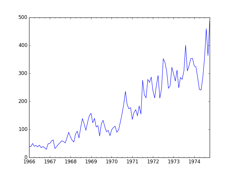
5.2 Line Plot

A line plot of a time series can provide a lot of insight into the problem.

The example below creates and shows a line plot of the dataset.

Run the example and review the plot. Note any obvious temporal structures in the series.

Some observations from the plot include:

• There is an increasing trend of robberies over time.
• There do not appear to be any obvious outliers.
• There are relatively large fluctuations from year to year, up and down.
• The fluctuations at later years appear larger than fluctuations at earlier years.
• The trend means the dataset is almost certainly non-stationary and the apparent change in fluctuation may also contribute.

Monthly Boston Robberies Line Plot

These simple observations suggest we may see benefit in modeling the trend and removing it from the time series.

Alternately, we could use differencing to make the series stationary for modeling. We may even need two levels of differencing if there is a growth trend in the fluctuations in later years.

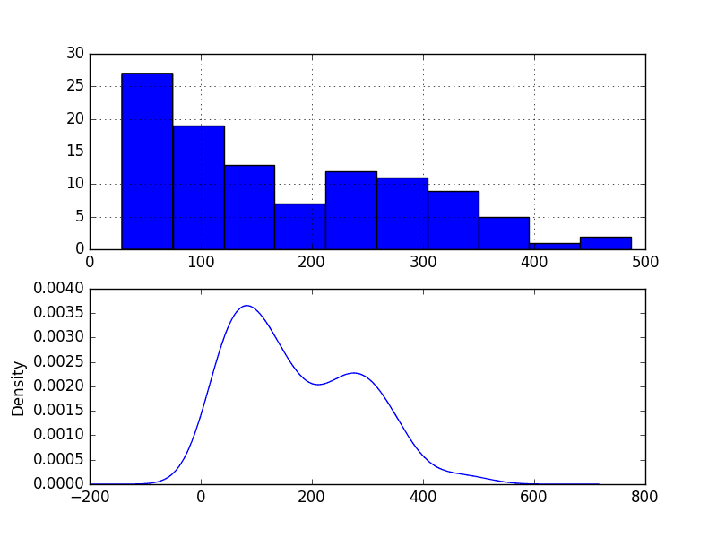
5.3 Density Plot

Reviewing plots of the density of observations can provide further insight into the structure of the data.

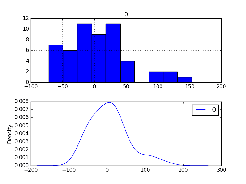
The example below creates a histogram and density plot of the observations without any temporal structure.

Run the example and review the plots.

Some observations from the plots include:

• The distribution is not Gaussian.
• The distribution is left shifted and may be exponential or a double Gaussian.

Monthly Boston Robberies Density Plot

We may see some benefit in exploring some power transforms of the data prior to modeling.

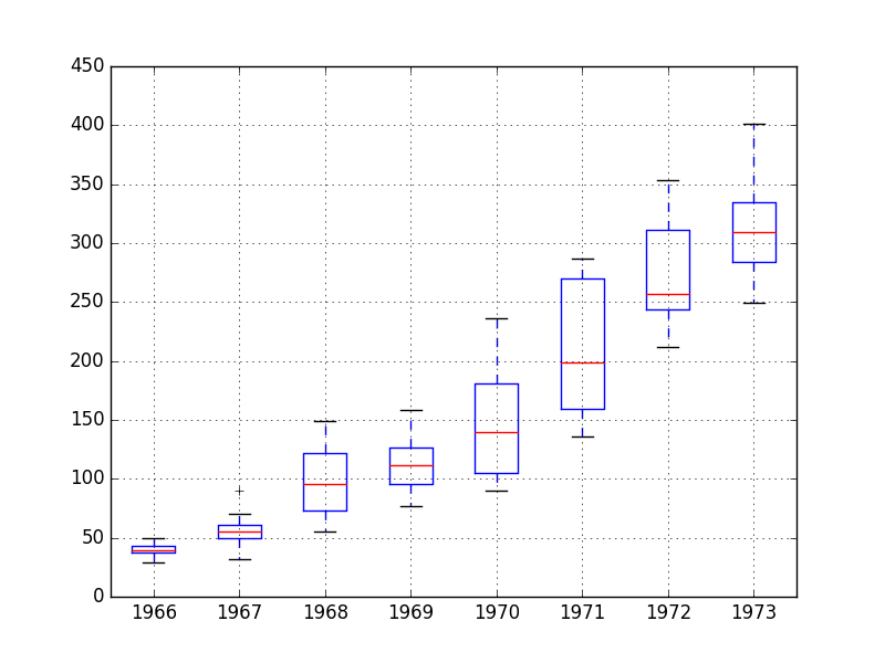
5.4 Box and Whisker Plots

We can group the monthly data by year and get an idea of the spread of observations for each year and how this may be changing.

We do expect to see some trend (increasing mean or median), but it may be interesting to see how the rest of the distribution may be changing.

The example below groups the observations by year and creates one box and whisker plot for each year of observations. The last year (1974) only contains 10 months and may not be a useful comparison with the other 12 months of observations in the other years. Therefore only data between 1966 and 1973 was plotted.

Running the example creates 8 box and whisker plots side-by-side, one for each of the 8 years of selected data.

Some observations from reviewing the plot include:

• The median values for each year (red line) show a trend that may not be linear.
• The spread, or middle 50% of the data (blue boxes), differ, but perhaps not consistently over time.
• The earlier years, perhaps first 2, are quite different from the rest of the dataset.

Monthly Boston Robberies Box and Whisker Plots

The observations suggest that the year-to-year fluctuations may not be systematic and hard to model. They also suggest that there may be some benefit in clipping the first two years of data from modeling if it is indeed quite different.

This yearly view of the data is an interesting avenue and could be pursued further by looking at summary statistics from year-to-year and changes in summary stats from year-to-year.

Next, we can start looking at predictive models of the series.

6. ARIMA Models

In this section, we will develop Autoregression Integrated Moving Average, or ARIMA, models for the problem.

We will approach this in four steps:

1. Developing a manually configured ARIMA model.
2. Using a grid search of ARIMA to find an optimized model.
3. Analysis of forecast residual errors to evaluate any bias in the model.
4. Explore improvements to the model using power transforms.

6.1 Manually Configured ARIMA

Nonseasonal ARIMA(p,d,q) requires three parameters and is traditionally configured manually.

Analysis of the time series data assumes that we are working with a stationary time series.

The time series is almost certainly non-stationary. We can make it stationary by first differencing the series and using a statistical test to confirm that the result is stationary.

The example below creates a stationary version of the series and saves it to file stationary.csv.

Running the example outputs the result of a statistical significance test of whether the series is stationary. Specifically, the augmented Dickey-Fuller test.

The results show that the test statistic value -3.980946 is smaller than the critical value at 5% of -2.893. This suggests that we can reject the null hypothesis with a significance level of less than 5% (i.e. a low probability that the result is a statistical fluke).

Rejecting the null hypothesis means that the process has no unit root, and in turn that the time series is stationary or does not have time-dependent structure.

This suggests that at least one level of differencing is required. The d parameter in our ARIMA model should at least be a value of 1.

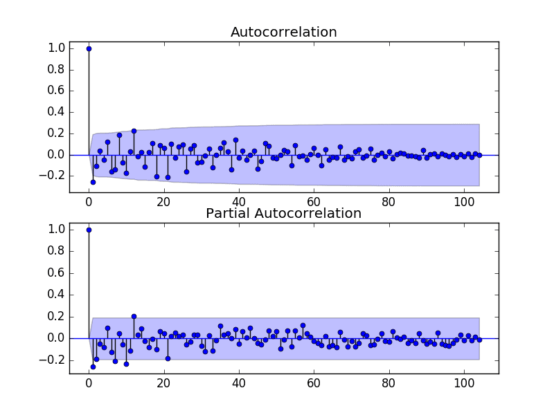
The next step is to select the lag values for the Autoregression (AR) and Moving Average (MA) parameters, p and q respectively.

We can do this by reviewing Autocorrelation Function (ACF) and Partial Autocorrelation Function (PACF) plots.

The example below creates ACF and PACF plots for the series.

Run the example and review the plots for insights into how to set the p and q variables for the ARIMA model.

Below are some observations from the plots.

• The ACF shows a significant lag for 1 month.
• The PACF shows a significant lag for perhaps 2 months, with significant lags spotty out to perhaps 12 months.
• Both the ACF and PACF show a drop-off at the same point, perhaps suggesting a mix of AR and MA.

A good starting point for the p and q values is 1 or 2.

Monthly Boston Robberies ACF and PACF Plots

This quick analysis suggests an ARIMA(1,1,2) on the raw data may be a good starting point.

Experimentation shows that this configuration of ARIMA does not converge and results in errors by the underlying library. Some experimentation shows that the model does not appear to be stable, with non-zero AR and MA orders defined at the same time.

The model can be simplified to ARIMA(0,1,2). The example below demonstrates the performance of this ARIMA model on the test harness.

Running this example results in an RMSE of 49.821, which is lower than the persistence model.

This is a good start, but we may be able to get improved results with a better configured ARIMA model.

6.2 Grid Search ARIMA Hyperparameters

Many ARIMA configurations are unstable on this dataset, but there may be other hyperparameters that result in a well-performing model.

In this section, we will search values of p, d, and q for combinations that do not result in error, and find the combination that results in the best performance. We will use a grid search to explore all combinations in a subset of integer values.

Specifically, we will search all combinations of the following parameters:

• p: 0 to 12.
• d: 0 to 3.
• q: 0 to 12.

This is (13 * 4 * 13), or 676, runs of the test harness and will take some time to execute.

The complete worked example with the grid search version of the test harness is listed below.

Running the example runs through all combinations and reports the results on those that converge without error.

The example takes a little less than 2 hours to run on modern hardware.

The results show that the best configuration discovered was ARIMA(0, 1, 2); coincidently, that was demonstrated in the previous section.

6.3 Review Residual Errors

A good final check of a model is to review residual forecast errors.

Ideally, the distribution of residual errors should be a Gaussian with a zero mean.

We can check this by plotting the residuals with a histogram and density plots.

The example below calculates the residual errors for predictions on the test set and creates these density plots.

Running the example creates the two plots.

The graphs suggest a Gaussian-like distribution with a longer right tail.

This is perhaps a sign that the predictions are biased, and in this case that perhaps a power-based transform of the raw data before modeling might be useful.

Residual Errors Density Plots

It is also a good idea to check the time series of the residual errors for any type of autocorrelation. If present, it would suggest that the model has more opportunity to model the temporal structure in the data.

The example below re-calculates the residual errors and creates ACF and PACF plots to check for any significant autocorrelation.

The results suggest that what little autocorrelation is present in the time series has been captured by the model.

Residual Errors ACF and PACF Plots

6.4 Box-Cox Transformed Dataset

The Box-Cox transform is a method that is able to evaluate a suite of power transforms, including, but not limited to, log, square root, and reciprocal transforms of the data.

The example below performs a log transform of the data and generates some plots to review the effect on the time series.

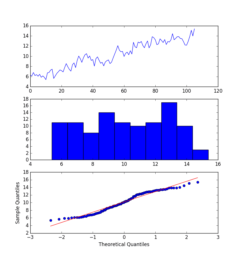
Running the example creates three graphs: a line chart of the transformed time series, a histogram showing the distribution of transformed values, and a Q-Q plot showing how the distribution of values compared to an idealized Gaussian distribution.

Some observations from these plots are follows:

• The large fluctuations have been removed from the line plot of the time series.
• The histogram shows a flatter or more uniform (well behaved) distribution of values.
• The Q-Q plot is reasonable, but still not a perfect fit for a Gaussian distribution.

BoxCox Transform Plots of Monthly Boston Robberies

Undoubtedly, the Box-Cox transform has done something to the time series and may be useful.

Before proceeding to test the ARIMA model with the transformed data, we must have a way to reverse the transform in order to convert predictions made with a model trained on the transformed data back into the original scale.

The boxcox() function used in the example finds an ideal lambda value by optimizing a cost function.

The lambda is used in the following function to transform the data:

This transform function can be reversed directly, as follows:

This inverse Box-Cox transform function can be implemented in Python as follows:

We can re-evaluate the ARIMA(0,1,2) model with the Box-Cox transform.

This involves first transforming the history prior to fitting the ARIMA model, then inverting the transform on the prediction before storing it for later comparison with the expected values.

The boxcox() function can fail. In practice, I have seen this and it appears to be signaled by a returned lambda value of less than -5. By convention, lambda values are evaluated between -5 and 5.

A check is added for a lambda value less than -5, and if this the case, a lambda value of 1 is assumed and the raw history is used to fit the model. A lambda value of 1 is the same as “no-transform” and therefore the inverse transform has no effect.

The complete example is listed below.

Running the example prints the predicted and expected value each iteration.

Note, you may see warnings when using the boxcox() transform function; for example:

These can be ignored for now.

The final RMSE of the model on the transformed data was 49.443. This is a smaller error than the ARIMA model on untransformed data, but only slightly, and it may or may not be statistically different.

We will use this model with the Box-Cox transform as the final model.

7. Model Validation

After models have been developed and a final model selected, it must be validated and finalized.

Validation is an optional part of the process, but one that provides a ‘last check’ to ensure we have not fooled or lied to ourselves.

This section includes the following steps:

1. Finalize Model: Train and save the final model.
2. Make Prediction: Load the finalized model and make a prediction.
3. Validate Model: Load and validate the final model.

7.1 Finalize Model

Finalizing the model involves fitting an ARIMA model on the entire dataset, in this case, on a transformed version of the entire dataset.

Once fit, the model can be saved to file for later use. Because a Box-Cox transform is also performed on the data, we need to know the chosen lambda so that any predictions from the model can be converted back to the original, untransformed scale.

The example below fits an ARIMA(0,1,2) model on the Box-Cox transform dataset and saves the whole fit object and the lambda value to file.

Running the example creates two local files:

• model.pkl This is the ARIMAResult object from the call to ARIMA.fit(). This includes the coefficients and all other internal data returned when fitting the model.
• model_lambda.npy This is the lambda value stored as a one-row, one-column NumPy array.

This is probably overkill and all that is really needed for operational use are the AR and MA coefficients from the model, the d parameter for the number of differences, perhaps the lag observations and model residuals, and the lambda value for the transform.

7.2 Make Prediction

A natural case may be to load the model and make a single forecast.

This is relatively straightforward and involves restoring the saved model and the lambda and calling the forecast() method.

The example below loads the model, makes a prediction for the next time step, inverses the Box-Cox transform, and prints the prediction.

Running the example prints the prediction of about 452.

If we peek inside validation.csv, we can see that the value on the first row for the next time period is 452. The model got it 100% correct, which is very impressive (or lucky).

7.3 Validate Model

We can load the model and use it in a pretend operational manner.

In the test harness section, we saved the final 12 months of the original dataset in a separate file to validate the final model.

We can load this validation.csv file now and use it see how well our model really is on “unseen” data.

There are two ways we might proceed:

• Load the model and use it to forecast the next 12 months. The forecast beyond the first one or two months will quickly start to degrade in skill.
• Load the model and use it in a rolling-forecast manner, updating the transform and model for each time step. This is the preferred method as it is how one would use this model in practice, as it would achieve the best performance.

As with model evaluation in previous sections, we will make predictions in a rolling-forecast manner. This means that we will step over lead times in the validation dataset and take the observations as an update to the history.

Running the example prints each prediction and expected value for the time steps in the validation dataset.

The final RMSE for the validation period is predicted at 53 robberies. This is not too different to the expected error of 49, but I would expect that it is also not too different from a simple persistence model.

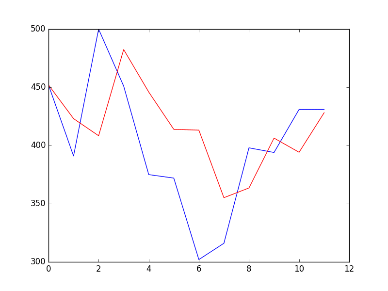
A plot of the predictions compared to the validation dataset is also provided.

The forecast does have the characteristic of a persistence forecast. This does suggest that although this time series does have an obvious trend, it is still a reasonably difficult problem.

Forecast for Validation Time Steps

Tutorial Extensions

This tutorial was not exhaustive; there may be more that you can do to improve the result.

This section lists some ideas.

• Statistical Significance Tests. Use a statistical test to check if the difference in results between different models is statistically significant. The Student t-test would be a good place to start.
• Grid Search with Data Transforms. Repeat the grid search in the ARIMA hyperparameters with the Box-Cox transform and see if a different and better set of parameters can be achieved.
• Inspect Residuals. Investigate the residual forecast errors on the final model with Box-Cox transforms to see if there is a further bias and/or autocorrelation that can be addressed.
• Lean Model Saving. Simplify model saving to only store the required coefficients rather than the entire ARIMAResults object.
• Manually Handle Trend. Model the trend directly with a linear or nonlinear model and explicitly remove it from the series. This may result in better performance if the trend is nonlinear and can be modeled better than the linear case.
• Confidence Interval. Display the confidence intervals for the predictions on the validation dataset.
• Data Selection. Consider modeling the problem without the first two years of data and see if this has an impact on forecast skill.

Did you implement any of these extensions? Were you able to get a better result?
Share your findings in the comments below.

Summary

In this tutorial, you discovered the steps and the tools for a time series forecasting project with Python.

We covered a lot of ground in this tutorial, specifically:

• How to develop a test harness with a performance measure and evaluation method and how to quickly develop a baseline forecast and skill.
• How to use time series analysis to raise ideas for how to best model the forecast problem.
• How to develop an ARIMA model, save it, and later load it to make predictions on new data.

How did you do? Do you have any questions about this tutorial?
Ask your questions in the comments below and I will do my best to answer.

Want to Develop Time Series Forecasts with Python?

Develop Your Own Forecasts in Minutes

...with just a few lines of python code

Discover how in my new Ebook:
Introduction to Time Series Forecasting With Python

It covers self-study tutorials and end-to-end projects on topics like: Loading data, visualization, modeling, algorithm tuning, and much more...

Finally Bring Time Series Forecasting to
Your Own Projects

Skip the Academics. Just Results.

See What's Inside