The Luong Attention Mechanism

The Luong attention sought to introduce several improvements over the Bahdanau model for neural machine translation, notably by introducing two new classes of attentional mechanisms: a global approach that attends to all source words and a local approach that only attends to a selected subset of words in predicting the target sentence. 

In this tutorial, you will discover the Luong attention mechanism for neural machine translation. 

After completing this tutorial, you will know:

• The operations performed by the Luong attention algorithm
• How the global and local attentional models work.
• How the Luong attention compares to the Bahdanau attention

Kick-start your project with my book Building Transformer Models with Attention. It provides self-study tutorials with working code to guide you into building a fully-working transformer model that can
translate sentences from one language to another...

Let’s get started. 

The Luong attention mechanism
Photo by Mike Nahlii, some rights reserved.

Tutorial Overview

This tutorial is divided into five parts; they are:

• Introduction to the Luong Attention
• The Luong Attention Algorithm
• The Global Attentional Model
• The Local Attentional Model
• Comparison to the Bahdanau Attention

Prerequisites

For this tutorial, we assume that you are already familiar with:

• The concept of attention
• The attention mechanism
• The Bahdanau attention mechanism

Introduction to the Luong Attention

Luong et al. (2015) inspire themselves from previous attention models to propose two attention mechanisms:

In this work, we design, with simplicity and effectiveness in mind, two novel types of attention-based models: a global approach which always attends to all source words and a local one that only looks at a subset of source words at a time.

– Effective Approaches to Attention-based Neural Machine Translation, 2015.

The global attentional model resembles the Bahdanau et al. (2014) model in attending to all source words but aims to simplify it architecturally. 

The local attentional model is inspired by the hard and soft attention models of Xu et al. (2016) and attends to only a few of the source positions. 

The two attentional models share many of the steps in their prediction of the current word but differ mainly in their computation of the context vector.

Let’s first take a look at the overarching Luong attention algorithm and then delve into the differences between the global and local attentional models afterward. 

The Luong Attention Algorithm

The attention algorithm of Luong et al. performs the following operations:

1. The encoder generates a set of annotations, $H = \mathbf{h}_i, i = 1, \dots, T$, from the input sentence. 

2. The current decoder hidden state is computed as: $\mathbf{s}_t = \text{RNN}_\text{decoder}(\mathbf{s}_{t-1}, y_{t-1})$. Here, $\mathbf{s}_{t-1}$ denotes the previous hidden decoder state and $y_{t-1}$ the previous decoder output. 

3. An alignment model, $a(.)$, uses the annotations and the current decoder hidden state to compute the alignment scores: $e_{t,i} = a(\mathbf{s}_t, \mathbf{h}_i)$. 

4. A softmax function is applied to the alignment scores, effectively normalizing them into weight values in a range between 0 and 1: $\alpha_{t,i} = \text{softmax}(e_{t,i})$.

5. Together with the previously computed annotations, these weights are used to generate a context vector through a weighted sum of the annotations: $\mathbf{c}_t = \sum^T_{i=1} \alpha_{t,i} \mathbf{h}_i$. 

6. An attentional hidden state is computed based on a weighted concatenation of the context vector and the current decoder hidden state: $\widetilde{\mathbf{s}}_t = \tanh(\mathbf{W_c} [\mathbf{c}_t \; ; \; \mathbf{s}_t])$.

7. The decoder produces a final output by feeding it a weighted attentional hidden state: $y_t = \text{softmax}(\mathbf{W}_y \widetilde{\mathbf{s}}_t)$. 

8. Steps 2-7 are repeated until the end of the sequence. 

The Global Attentional Model

The global attentional model considers all the source words in the input sentence when generating the alignment scores and, eventually, when computing the context vector. 

The idea of a global attentional model is to consider all the hidden states of the encoder when deriving the context vector, $\mathbf{c}_t$.

– Effective Approaches to Attention-based Neural Machine Translation, 2015.

In order to do so, Luong et al. propose three alternative approaches for computing the alignment scores. The first approach is similar to Bahdanau’s. It is based upon the concatenation of $\mathbf{s}_t$ and $\mathbf{h}_i$, while the second and third approaches implement multiplicative attention (in contrast to Bahdanau’s additive attention):

1. $$a(\mathbf{s}_t, \mathbf{h}_i) = \mathbf{v}_a^T \tanh(\mathbf{W}_a [\mathbf{s}_t \; ; \; \mathbf{h}_i)]$$

2. $$a(\mathbf{s}_t, \mathbf{h}_i) = \mathbf{s}^T_t \mathbf{h}_i$$

3. $$a(\mathbf{s}_t, \mathbf{h}_i) = \mathbf{s}^T_t \mathbf{W}_a \mathbf{h}_i$$

Here, $\mathbf{W}_a$ is a trainable weight matrix, and similarly, $\mathbf{v}_a$ is a weight vector.

Intuitively, the use of the dot product in multiplicative attention can be interpreted as providing a similarity measure between the vectors, $\mathbf{s}_t$ and $\mathbf{h}_i$, under consideration. 

… if the vectors are similar (that is, aligned), the result of the multiplication will be a large value and the attention will be focused on the current t,i relationship.

– Advanced Deep Learning with Python, 2019.

The resulting alignment vector, $\mathbf{e}_t$, is of a variable length according to the number of source words. 

The Local Attentional Model

In attending to all source words, the global attentional model is computationally expensive and could potentially become impractical for translating longer sentences. 

The local attentional model seeks to address these limitations by focusing on a smaller subset of the source words to generate each target word. In order to do so, it takes inspiration from the hard and soft attention models of the image caption generation work of Xu et al. (2016):

• Soft attention is equivalent to the global attention approach, where weights are softly placed over all the source image patches. Hence, soft attention considers the source image in its entirety. 

• Hard attention attends to a single image patch at a time.

The local attentional model of Luong et al. generates a context vector by computing a weighted average over the set of annotations, $\mathbf{h}_i$, within a window centered over an aligned position, $p_t$:

$$[p_t – D, p_t + D]$$

While a value for $D$ is selected empirically, Luong et al. consider two approaches in computing a value for $p_t$:

1. Monotonic alignment: where the source and target sentences are assumed to be monotonically aligned and, hence, $p_t = t$.

2. Predictive alignment: where a prediction of the aligned position is based upon trainable model parameters, $\mathbf{W}_p$ and $\mathbf{v}_p$, and the source sentence length, $S$:

$$p_t = S \cdot \text{sigmoid}(\mathbf{v}^T_p \tanh(\mathbf{W}_p, \mathbf{s}_t))$$

A Gaussian distribution is centered around $p_t$ when computing the alignment weights to favor source words nearer to the window center. 

This time round, the resulting alignment vector, $\mathbf{e}_t$, has a fixed length of $2D + 1$.

Kick-start your project with my book Building Transformer Models with Attention. It provides self-study tutorials with working code to guide you into building a fully-working transformer model that can
translate sentences from one language to another...

Comparison to the Bahdanau Attention

The Bahdanau model and the global attention approach of Luong et al. are mostly similar, but there are key differences between the two:

While our global attention approach is similar in spirit to the model proposed by Bahdanau et al. (2015), there are several key differences which reflect how we have both simplified and generalized from the original model.

– Effective Approaches to Attention-based Neural Machine Translation, 2015.

1. Most notably, the computation of the alignment scores, $e_t$, in the Luong global attentional model depends on the current decoder hidden state, $\mathbf{s}_t$, rather than on the previous hidden state, $\mathbf{s}_{t-1}$, as in the Bahdanau attention. 

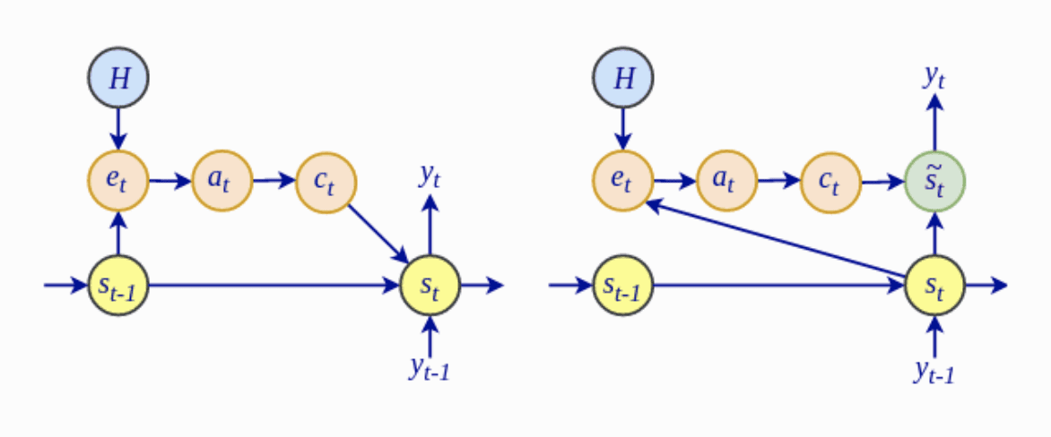
The Bahdanau architecture (left) vs. the Luong architecture (right)
Taken from “Advanced Deep Learning with Python“

2. Luong et al. drop the bidirectional encoder used by the Bahdanau model and instead utilize the hidden states at the top LSTM layers for both the encoder and decoder. 

3. The global attentional model of Luong et al. investigates the use of multiplicative attention as an alternative to the Bahdanau additive attention. 

Further Reading

This section provides more resources on the topic if you are looking to go deeper.

Books

• Advanced Deep Learning with Python, 2019.

Papers

• Effective Approaches to Attention-based Neural Machine Translation, 2015.

Summary

In this tutorial, you discovered the Luong attention mechanism for neural machine translation. 

Specifically, you learned:

• The operations performed by the Luong attention algorithm
• How the global and local attentional models work 
• How the Luong attention compares to the Bahdanau attention

Do you have any questions?
Ask your questions in the comments below, and I will do my best to answer.

Learn Transformers and Attention!

Teach your deep learning model to read a sentence

...using transformer models with attention

Discover how in my new Ebook:
Building Transformer Models with Attention

It provides self-study tutorials with working code to guide you into building a fully-working transformer models that can
translate sentences from one language to another...

Give magical power of understanding human language for
Your Projects

See What's Inside