We have previously seen how to train the Transformer model for neural machine translation. Before moving on to inferencing the trained model, let us first explore how to modify the training code slightly to be able to plot the training and validation loss curves that can be generated during the learning process.
The training and validation loss values provide important information because they give us a better insight into how the learning performance changes over the number of epochs and help us diagnose any problems with learning that can lead to an underfit or an overfit model. They will also inform us about the epoch with which to use the trained model weights at the inferencing stage.
In this tutorial, you will discover how to plot the training and validation loss curves for the Transformer model.
After completing this tutorial, you will know:
- How to modify the training code to include validation and test splits, in addition to a training split of the dataset
- How to modify the training code to store the computed training and validation loss values, as well as the trained model weights
- How to plot the saved training and validation loss curves
Kick-start your project with my book Building Transformer Models with Attention. It provides self-study tutorials with working code to guide you into building a fully-working transformer model that can
translate sentences from one language to another...
Let’s get started.

Plotting the training and validation loss curves for the Transformer model
Photo by Jack Anstey, some rights reserved.
Tutorial Overview
This tutorial is divided into four parts; they are:
- Recap of the Transformer Architecture
- Preparing the Training, Validation, and Testing Splits of the Dataset
- Training the Transformer Model
- Plotting the Training and Validation Loss Curves
Prerequisites
For this tutorial, we assume that you are already familiar with:
- The theory behind the Transformer model
- An implementation of the Transformer model
- Training the Transformer model
Recap of the Transformer Architecture
Recall having seen that the Transformer architecture follows an encoder-decoder structure. The encoder, on the left-hand side, is tasked with mapping an input sequence to a sequence of continuous representations; the decoder, on the right-hand side, receives the output of the encoder together with the decoder output at the previous time step to generate an output sequence.
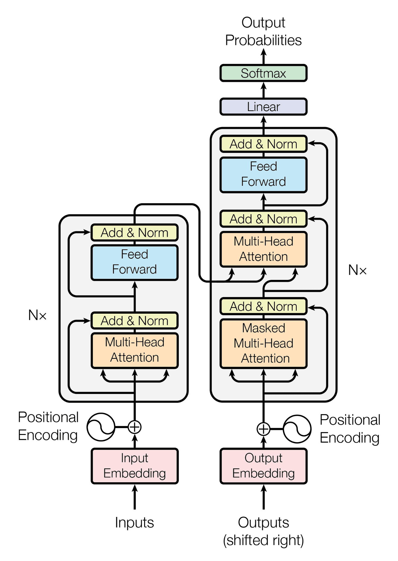
The encoder-decoder structure of the Transformer architecture
Taken from “Attention Is All You Need“
In generating an output sequence, the Transformer does not rely on recurrence and convolutions.
You have seen how to train the complete Transformer model, and you shall now see how to generate and plot the training and validation loss values that will help you diagnose the model’s learning performance.
Want to Get Started With Building Transformer Models with Attention?
Take my free 12-day email crash course now (with sample code).
Click to sign-up and also get a free PDF Ebook version of the course.
Preparing the Training, Validation, and Testing Splits of the Dataset
In order to be able to include validation and test splits of the data, you will modify the code that prepares the dataset by introducing the following lines of code, which:
- Specify the size of the validation data split. This, in turn, determines the size of the training and test splits of the data, which we will be dividing into a ratio of 80:10:10 for the training, validation, and test sets, respectively:
|
1 |
self.val_split = 0.1 # Ratio of the validation data split |
- Split the dataset into validation and test sets in addition to the training set:
|
1 2 |
val = dataset[int(self.n_sentences * self.train_split):int(self.n_sentences * (1-self.val_split))] test = dataset[int(self.n_sentences * (1 - self.val_split)):] |
- Prepare the validation data by tokenizing, padding, and converting to a tensor. For this purpose, you will collect these operations into a function called
encode_pad, as shown in the complete code listing below. This will avoid excessive repetition of code when performing these operations on the training data as well:
|
1 2 |
valX = self.encode_pad(val[:, 0], enc_tokenizer, enc_seq_length) valY = self.encode_pad(val[:, 1], dec_tokenizer, dec_seq_length) |
- Save the encoder and decoder tokenizers into pickle files and the test dataset into a text file to be used later during the inferencing stage:
|
1 2 3 |
self.save_tokenizer(enc_tokenizer, 'enc') self.save_tokenizer(dec_tokenizer, 'dec') savetxt('test_dataset.txt', test, fmt='%s') |
The complete code listing is now updated as follows:
|
1 2 3 4 5 6 7 8 9 10 11 12 13 14 15 16 17 18 19 20 21 22 23 24 25 26 27 28 29 30 31 32 33 34 35 36 37 38 39 40 41 42 43 44 45 46 47 48 49 50 51 52 53 54 55 56 57 58 59 60 61 62 63 64 65 66 67 68 69 70 71 72 73 74 75 76 77 78 79 80 81 82 83 84 85 86 87 88 89 |
from pickle import load, dump, HIGHEST_PROTOCOL from numpy.random import shuffle from numpy import savetxt from keras.preprocessing.text import Tokenizer from keras.preprocessing.sequence import pad_sequences from tensorflow import convert_to_tensor, int64 class PrepareDataset: def __init__(self, **kwargs): super(PrepareDataset, self).__init__(**kwargs) self.n_sentences = 15000 # Number of sentences to include in the dataset self.train_split = 0.8 # Ratio of the training data split self.val_split = 0.1 # Ratio of the validation data split # Fit a tokenizer def create_tokenizer(self, dataset): tokenizer = Tokenizer() tokenizer.fit_on_texts(dataset) return tokenizer def find_seq_length(self, dataset): return max(len(seq.split()) for seq in dataset) def find_vocab_size(self, tokenizer, dataset): tokenizer.fit_on_texts(dataset) return len(tokenizer.word_index) + 1 # Encode and pad the input sequences def encode_pad(self, dataset, tokenizer, seq_length): x = tokenizer.texts_to_sequences(dataset) x = pad_sequences(x, maxlen=seq_length, padding='post') x = convert_to_tensor(x, dtype=int64) return x def save_tokenizer(self, tokenizer, name): with open(name + '_tokenizer.pkl', 'wb') as handle: dump(tokenizer, handle, protocol=HIGHEST_PROTOCOL) def __call__(self, filename, **kwargs): # Load a clean dataset clean_dataset = load(open(filename, 'rb')) # Reduce dataset size dataset = clean_dataset[:self.n_sentences, :] # Include start and end of string tokens for i in range(dataset[:, 0].size): dataset[i, 0] = "<START> " + dataset[i, 0] + " <EOS>" dataset[i, 1] = "<START> " + dataset[i, 1] + " <EOS>" # Random shuffle the dataset shuffle(dataset) # Split the dataset in training, validation and test sets train = dataset[:int(self.n_sentences * self.train_split)] val = dataset[int(self.n_sentences * self.train_split):int(self.n_sentences * (1-self.val_split))] test = dataset[int(self.n_sentences * (1 - self.val_split)):] # Prepare tokenizer for the encoder input enc_tokenizer = self.create_tokenizer(dataset[:, 0]) enc_seq_length = self.find_seq_length(dataset[:, 0]) enc_vocab_size = self.find_vocab_size(enc_tokenizer, train[:, 0]) # Prepare tokenizer for the decoder input dec_tokenizer = self.create_tokenizer(dataset[:, 1]) dec_seq_length = self.find_seq_length(dataset[:, 1]) dec_vocab_size = self.find_vocab_size(dec_tokenizer, train[:, 1]) # Encode and pad the training input trainX = self.encode_pad(train[:, 0], enc_tokenizer, enc_seq_length) trainY = self.encode_pad(train[:, 1], dec_tokenizer, dec_seq_length) # Encode and pad the validation input valX = self.encode_pad(val[:, 0], enc_tokenizer, enc_seq_length) valY = self.encode_pad(val[:, 1], dec_tokenizer, dec_seq_length) # Save the encoder tokenizer self.save_tokenizer(enc_tokenizer, 'enc') # Save the decoder tokenizer self.save_tokenizer(dec_tokenizer, 'dec') # Save the testing dataset into a text file savetxt('test_dataset.txt', test, fmt='%s') return trainX, trainY, valX, valY, train, val, enc_seq_length, dec_seq_length, enc_vocab_size, dec_vocab_size |
Training the Transformer Model
We shall introduce similar modifications to the code that trains the Transformer model to:
- Prepare the validation dataset batches:
|
1 2 |
val_dataset = data.Dataset.from_tensor_slices((valX, valY)) val_dataset = val_dataset.batch(batch_size) |
- Monitor the validation loss metric:
|
1 |
val_loss = Mean(name='val_loss') |
- Initialize dictionaries to store the training and validation losses and eventually store the loss values in the respective dictionaries:
|
1 2 3 4 5 |
train_loss_dict = {} val_loss_dict = {} train_loss_dict[epoch] = train_loss.result() val_loss_dict[epoch] = val_loss.result() |
- Compute the validation loss:
|
1 2 |
loss = loss_fcn(decoder_output, prediction) val_loss(loss) |
- Save the trained model weights at every epoch. You will use these at the inferencing stage to investigate the differences in results that the model produces at different epochs. In practice, it would be more efficient to include a callback method that halts the training process based on the metrics that are being monitored during training and only then save the model weights:
|
1 2 |
# Save the trained model weights training_model.save_weights("weights/wghts" + str(epoch + 1) + ".ckpt") |
- Finally, save the training and validation loss values into pickle files:
|
1 2 3 4 5 |
with open('./train_loss.pkl', 'wb') as file: dump(train_loss_dict, file) with open('./val_loss.pkl', 'wb') as file: dump(val_loss_dict, file) |
The modified code listing now becomes:
|
1 2 3 4 5 6 7 8 9 10 11 12 13 14 15 16 17 18 19 20 21 22 23 24 25 26 27 28 29 30 31 32 33 34 35 36 37 38 39 40 41 42 43 44 45 46 47 48 49 50 51 52 53 54 55 56 57 58 59 60 61 62 63 64 65 66 67 68 69 70 71 72 73 74 75 76 77 78 79 80 81 82 83 84 85 86 87 88 89 90 91 92 93 94 95 96 97 98 99 100 101 102 103 104 105 106 107 108 109 110 111 112 113 114 115 116 117 118 119 120 121 122 123 124 125 126 127 128 129 130 131 132 133 134 135 136 137 138 139 140 141 142 143 144 145 146 147 148 149 150 151 152 153 154 155 156 157 158 159 160 161 162 163 164 165 166 167 168 169 170 171 172 173 174 175 176 177 178 179 180 181 182 183 184 185 186 187 188 189 190 191 192 193 194 195 |
from tensorflow.keras.optimizers import Adam from tensorflow.keras.optimizers.schedules import LearningRateSchedule from tensorflow.keras.metrics import Mean from tensorflow import data, train, math, reduce_sum, cast, equal, argmax, float32, GradientTape, function from keras.losses import sparse_categorical_crossentropy from model import TransformerModel from prepare_dataset import PrepareDataset from time import time from pickle import dump # Define the model parameters h = 8 # Number of self-attention heads d_k = 64 # Dimensionality of the linearly projected queries and keys d_v = 64 # Dimensionality of the linearly projected values d_model = 512 # Dimensionality of model layers' outputs d_ff = 2048 # Dimensionality of the inner fully connected layer n = 6 # Number of layers in the encoder stack # Define the training parameters epochs = 20 batch_size = 64 beta_1 = 0.9 beta_2 = 0.98 epsilon = 1e-9 dropout_rate = 0.1 # Implementing a learning rate scheduler class LRScheduler(LearningRateSchedule): def __init__(self, d_model, warmup_steps=4000, **kwargs): super(LRScheduler, self).__init__(**kwargs) self.d_model = cast(d_model, float32) self.warmup_steps = warmup_steps def __call__(self, step_num): # Linearly increasing the learning rate for the first warmup_steps, and decreasing it thereafter arg1 = step_num ** -0.5 arg2 = step_num * (self.warmup_steps ** -1.5) return (self.d_model ** -0.5) * math.minimum(arg1, arg2) # Instantiate an Adam optimizer optimizer = Adam(LRScheduler(d_model), beta_1, beta_2, epsilon) # Prepare the training dataset dataset = PrepareDataset() trainX, trainY, valX, valY, train_orig, val_orig, enc_seq_length, dec_seq_length, enc_vocab_size, dec_vocab_size = dataset('english-german.pkl') print(enc_seq_length, dec_seq_length, enc_vocab_size, dec_vocab_size) # Prepare the training dataset batches train_dataset = data.Dataset.from_tensor_slices((trainX, trainY)) train_dataset = train_dataset.batch(batch_size) # Prepare the validation dataset batches val_dataset = data.Dataset.from_tensor_slices((valX, valY)) val_dataset = val_dataset.batch(batch_size) # Create model training_model = TransformerModel(enc_vocab_size, dec_vocab_size, enc_seq_length, dec_seq_length, h, d_k, d_v, d_model, d_ff, n, dropout_rate) # Defining the loss function def loss_fcn(target, prediction): # Create mask so that the zero padding values are not included in the computation of loss padding_mask = math.logical_not(equal(target, 0)) padding_mask = cast(padding_mask, float32) # Compute a sparse categorical cross-entropy loss on the unmasked values loss = sparse_categorical_crossentropy(target, prediction, from_logits=True) * padding_mask # Compute the mean loss over the unmasked values return reduce_sum(loss) / reduce_sum(padding_mask) # Defining the accuracy function def accuracy_fcn(target, prediction): # Create mask so that the zero padding values are not included in the computation of accuracy padding_mask = math.logical_not(equal(target, 0)) # Find equal prediction and target values, and apply the padding mask accuracy = equal(target, argmax(prediction, axis=2)) accuracy = math.logical_and(padding_mask, accuracy) # Cast the True/False values to 32-bit-precision floating-point numbers padding_mask = cast(padding_mask, float32) accuracy = cast(accuracy, float32) # Compute the mean accuracy over the unmasked values return reduce_sum(accuracy) / reduce_sum(padding_mask) # Include metrics monitoring train_loss = Mean(name='train_loss') train_accuracy = Mean(name='train_accuracy') val_loss = Mean(name='val_loss') # Create a checkpoint object and manager to manage multiple checkpoints ckpt = train.Checkpoint(model=training_model, optimizer=optimizer) ckpt_manager = train.CheckpointManager(ckpt, "./checkpoints", max_to_keep=None) # Initialise dictionaries to store the training and validation losses train_loss_dict = {} val_loss_dict = {} # Speeding up the training process @function def train_step(encoder_input, decoder_input, decoder_output): with GradientTape() as tape: # Run the forward pass of the model to generate a prediction prediction = training_model(encoder_input, decoder_input, training=True) # Compute the training loss loss = loss_fcn(decoder_output, prediction) # Compute the training accuracy accuracy = accuracy_fcn(decoder_output, prediction) # Retrieve gradients of the trainable variables with respect to the training loss gradients = tape.gradient(loss, training_model.trainable_weights) # Update the values of the trainable variables by gradient descent optimizer.apply_gradients(zip(gradients, training_model.trainable_weights)) train_loss(loss) train_accuracy(accuracy) for epoch in range(epochs): train_loss.reset_states() train_accuracy.reset_states() val_loss.reset_states() print("\nStart of epoch %d" % (epoch + 1)) start_time = time() # Iterate over the dataset batches for step, (train_batchX, train_batchY) in enumerate(train_dataset): # Define the encoder and decoder inputs, and the decoder output encoder_input = train_batchX[:, 1:] decoder_input = train_batchY[:, :-1] decoder_output = train_batchY[:, 1:] train_step(encoder_input, decoder_input, decoder_output) if step % 50 == 0: print(f'Epoch {epoch + 1} Step {step} Loss {train_loss.result():.4f} Accuracy {train_accuracy.result():.4f}') # Run a validation step after every epoch of training for val_batchX, val_batchY in val_dataset: # Define the encoder and decoder inputs, and the decoder output encoder_input = val_batchX[:, 1:] decoder_input = val_batchY[:, :-1] decoder_output = val_batchY[:, 1:] # Generate a prediction prediction = training_model(encoder_input, decoder_input, training=False) # Compute the validation loss loss = loss_fcn(decoder_output, prediction) val_loss(loss) # Print epoch number and accuracy and loss values at the end of every epoch print("Epoch %d: Training Loss %.4f, Training Accuracy %.4f, Validation Loss %.4f" % (epoch + 1, train_loss.result(), train_accuracy.result(), val_loss.result())) # Save a checkpoint after every epoch if (epoch + 1) % 1 == 0: save_path = ckpt_manager.save() print("Saved checkpoint at epoch %d" % (epoch + 1)) # Save the trained model weights training_model.save_weights("weights/wghts" + str(epoch + 1) + ".ckpt") train_loss_dict[epoch] = train_loss.result() val_loss_dict[epoch] = val_loss.result() # Save the training loss values with open('./train_loss.pkl', 'wb') as file: dump(train_loss_dict, file) # Save the validation loss values with open('./val_loss.pkl', 'wb') as file: dump(val_loss_dict, file) print("Total time taken: %.2fs" % (time() - start_time)) |
Plotting the Training and Validation Loss Curves
In order to be able to plot the training and validation loss curves, you will first load the pickle files containing the training and validation loss dictionaries that you saved when training the Transformer model earlier.
Then you will retrieve the training and validation loss values from the respective dictionaries and graph them on the same plot.
The code listing is as follows, which you should save into a separate Python script:
|
1 2 3 4 5 6 7 8 9 10 11 12 13 14 15 16 17 18 19 20 21 22 23 24 25 26 27 28 29 30 |
from pickle import load from matplotlib.pylab import plt from numpy import arange # Load the training and validation loss dictionaries train_loss = load(open('train_loss.pkl', 'rb')) val_loss = load(open('val_loss.pkl', 'rb')) # Retrieve each dictionary's values train_values = train_loss.values() val_values = val_loss.values() # Generate a sequence of integers to represent the epoch numbers epochs = range(1, 21) # Plot and label the training and validation loss values plt.plot(epochs, train_values, label='Training Loss') plt.plot(epochs, val_values, label='Validation Loss') # Add in a title and axes labels plt.title('Training and Validation Loss') plt.xlabel('Epochs') plt.ylabel('Loss') # Set the tick locations plt.xticks(arange(0, 21, 2)) # Display the plot plt.legend(loc='best') plt.show() |
Running the code above generates a similar plot of the training and validation loss curves to the one below:

Line plots of the training and validation loss values over several training epochs
Note that although you might see similar loss curves, they might not necessarily be identical to the ones above. This is because you are training the Transformer model from scratch, and the resulting training and validation loss values depend on the random initialization of the model weights.
Nonetheless, these loss curves give us a better insight into how the learning performance changes over the number of epochs and help us diagnose any problems with learning that can lead to an underfit or an overfit model.
For more details on using the training and validation loss curves to diagnose the learning performance of a model, you can refer to this tutorial by Jason Brownlee.
Further Reading
This section provides more resources on the topic if you are looking to go deeper.
Books
Papers
Websites
- How to use Learning Curves to Diagnose Machine Learning Model Performance, https://machinelearningmastery.com/learning-curves-for-diagnosing-machine-learning-model-performance/
Summary
In this tutorial, you discovered how to plot the training and validation loss curves for the Transformer model.
Specifically, you learned:
- How to modify the training code to include validation and test splits, in addition to a training split of the dataset
- How to modify the training code to store the computed training and validation loss values, as well as the trained model weights
- How to plot the saved training and validation loss curves
Do you have any questions?
Ask your questions in the comments below, and I will do my best to answer.
Learn Transformers and Attention!
Teach your deep learning model to read a sentence
...using transformer models with attention
Discover how in my new Ebook:
Building Transformer Models with Attention
It provides self-study tutorials with working code to guide you into building a fully-working transformer models that can
translate sentences from one language to another...


To get this to work, I had to cast the two items to a list (lines 6 & 7), like this:
# Retrieve each dictionary’s values
train_values = list(train_loss.values())
val_values = list(val_loss.values())
Great series, thanks!
How can plot accuracy for each individual category in classifiction of image after trainnig
Hi khatija…The following resource may be of interest:
https://machinelearningmastery.com/learning-curves-for-diagnosing-machine-learning-model-performance/
Hi, thanks so much. I am trying to adapt this for pytorch. Please how do I define the weights
Hi Olufunke…The following discussions may be of interest:
https://stackoverflow.com/questions/74754493/plot-training-and-validation-loss-in-pytorch
https://medium.datadriveninvestor.com/visualizing-training-and-validation-loss-in-real-time-using-pytorch-and-bokeh-5522401bc9dd
Thank you for the excellent series! It has been very helpful.
I think there are two minor typos in this post:
– Line 70 in the code for prepare-dataset should have “dataset” instead of “train”.
– Line 51 in the code for training is missing “-both” in the name for the utilized dataset.
After making these modifications I got the same validation loss curve.
Thank you again and all the best!
Hi Oliver…You are very welcome! Thank you for your feedback!