Normal Bayes Classifier for Image Segmentation Using OpenCV

By Stefania Cristina on January 30, 2024 in OpenCV 0

The Naive Bayes algorithm is a simple but powerful technique for supervised machine learning. Its Gaussian variant is implemented in the OpenCV library.

In this tutorial, you will learn how to apply OpenCV’s normal Bayes algorithm, first on a custom two-dimensional dataset and subsequently for segmenting an image.

After completing this tutorial, you will know:

Several of the most important points in applying the Bayes theorem to machine learning.
How to use the normal Bayes algorithm on a custom dataset in OpenCV.
How to use the normal Bayes algorithm to segment an image in OpenCV.

Kick-start your project with my book Machine Learning in OpenCV. It provides self-study tutorials with working code.

Let’s get started.

Normal Bayes Classifier for Image Segmentation Using OpenCV
Photo by Fabian Irsara, some rights reserved.

Tutorial Overview

This tutorial is divided into three parts; they are:

Reminder of the Bayes Theorem As Applied to Machine Learning
Discovering Bayes Classification in OpenCV
Image Segmentation Using a Normal Bayes Classifier

Reminder of the Bayes Theorem As Applied to Machine Learning

This tutorial by Jason Brownlee gives an in-depth explanation of Bayes Theorem for machine learning, so let’s first start with brushing up on some of the most important points from his tutorial:

The Bayes Theorem is useful in machine learning because it provides a statistical model to formulate the relationship between data and a hypothesis.

Expressed as $P(h | D) = P(D | h) * P(h) / P(D)$, the Bayes Theorem states that the probability of a given hypothesis being true (denoted by $P(h | D)$ and known as the posterior probability of the hypothesis) can be calculated in terms of:

- The probability of observing the data given the hypothesis (denoted by $P(D | h)$ and known as the likelihood).
- The probability of the hypothesis being true, independently of the data (denoted by $P(h)$ and known as the prior probability of the hypothesis).
- The probability of observing the data independently of the hypothesis (denoted by $P(D)$ and known as the evidence).

The Bayes Theorem assumes that every variable (or feature) making up the input data, $D$, depends on all the other variables (or features).

Within the context of data classification, the Bayes Theorem may be applied to the problem of calculating the conditional probability of a class label given a data sample: $P(class | data) = P(data | class) * P(class) / P(data)$, where the class label now substitutes the hypothesis. The evidence, $P(data)$, is a constant and can be dropped.

In the formulation of the problem as outlined in the bullet point above, the estimation of the likelihood, $P(data | class)$, can be difficult because it requires that the number of data samples is sufficiently large to contain all possible combinations of variables (or features) for each class. This is seldom the case, especially with high-dimensional data with many variables.

The formulation above can be simplified into what is known as Naive Bayes, where each input variable is treated separately: $P(class | X_1, X_2, \dots, X_n) = P(X_1 | class) * P(X_2 | class) * \dots * P(X_n | class) * P(class)$

The Naive Bayes estimation changes the formulation from a dependent conditional probability model to an independent conditional probability model, where the input variables (or features) are now assumed to be independent. This assumption rarely holds with real-world data, hence the name naive.

Discovering Bayes Classification in OpenCV

Suppose the input data we are working with is continuous. In that case, it may be modeled using a continuous probability distribution, such as a Gaussian (or normal) distribution, where the data belonging to each class is modeled by its mean and standard deviation.

The Bayes classifier implemented in OpenCV is a normal Bayes classifier (also commonly known as Gaussian Naive Bayes), which assumes that the input features from each class are normally distributed.

This simple classification model assumes that feature vectors from each class are normally distributed (though, not necessarily independently distributed).

– OpenCV, Machine Learning Overview, 2023.

To discover how to use the normal Bayes classifier in OpenCV, let’s start by testing it on a simple two-dimensional dataset, as we did in previous tutorials.

Want to Get Started With Machine Learning with OpenCV?

Take my free email crash course now (with sample code).

Click to sign-up and also get a free PDF Ebook version of the course.

For this purpose, let’s generate a dataset consisting of 100 data points (specified by n_samples), which are equally divided into 2 Gaussian clusters (identified by centers) having a standard deviation set to 1.5 (specified by cluster_std). Let’s also define a value for random_state to be able to replicate the results:

# Generating a dataset of 2D data points and their ground truth labels
x, y_true = make_blobs(n_samples=100, centers=2, cluster_std=1.5, random_state=15)

# Plotting the dataset
scatter(x[:, 0], x[:, 1], c=y_true)
show()

# Generating a dataset of 2D data points and their ground truth labels

x, y_true = make_blobs(n_samples=100, centers=2, cluster_std=1.5, random_state=15)

# Plotting the dataset

scatter(x[:, 0], x[:, 1], c=y_true)

show()

The code above should generate the following plot of data points:

Scatter Plot of Dataset Consisting of 2 Gaussian Clusters

We shall then split this dataset, allocating 80% of the data to the training set and the remaining 20% to the test set:

# Split the data into training and testing sets
x_train, x_test, y_train, y_test = ms.train_test_split(x, y_true, test_size=0.2, random_state=10)

1 2	# Split the data into training and testing sets x_train, x_test, y_train, y_test = ms.train_test_split(x, y_true, test_size=0.2, random_state=10)

Following this, we will create the normal Bayes classifier and proceed with training and testing it on the dataset values after having type cast to 32-bit float:

# Create a new Normal Bayes Classifier
norm_bayes = ml.NormalBayesClassifier_create()

# Train the classifier on the training data
norm_bayes.train(x_train.astype(float32), ml.ROW_SAMPLE, y_train)

# Generate a prediction from the trained classifier
ret, y_pred, y_probs = norm_bayes.predictProb(x_test.astype(float32))

# Create a new Normal Bayes Classifier

norm_bayes = ml.NormalBayesClassifier_create()

# Train the classifier on the training data

norm_bayes.train(x_train.astype(float32), ml.ROW_SAMPLE, y_train)

# Generate a prediction from the trained classifier

ret, y_pred, y_probs = norm_bayes.predictProb(x_test.astype(float32))

By making use of the predictProb method, we will obtain the predicted class for each input vector (with each vector being stored on each row of the array fed into the normal Bayes classifier) and the output probabilities.

In the code above, the predicted classes are stored in y_pred, whereas y_probs is an array with as many columns as classes (two in this case) that holds the probability value of each input vector belonging to each class under consideration. It would make sense that the output probability values the classifier returns for each input vector sum up to one. However, this may not necessarily be the case because the probability values the classifier returns are not normalized by the evidence, $P(data)$, which we have removed from the denominator, as explained in the previous section.

Instead, what is being reported is a likelihood, which is basically the numerator of the conditional probability equation, p(C) p(M | C). The denominator, p(M), does not need to be computed.

– Machine Learning for OpenCV, 2017.

Nonetheless, whether the values are normalized or not, the class prediction for each input vector may be found by identifying the class with the highest probability value.

The code listing so far is the following:

from sklearn.datasets import make_blobs
from sklearn import model_selection as ms
from numpy import float32
from matplotlib.pyplot import scatter, show
from cv2 import ml

# Generate a dataset of 2D data points and their ground truth labels
x, y_true = make_blobs(n_samples=100, centers=2, cluster_std=1.5, random_state=15)

# Plot the dataset
scatter(x[:, 0], x[:, 1], c=y_true)
show()

# Split the data into training and testing sets
x_train, x_test, y_train, y_test = ms.train_test_split(x, y_true, test_size=0.2, random_state=10)

# Create a new Normal Bayes Classifier
norm_bayes = ml.NormalBayesClassifier_create()

# Train the classifier on the training data
norm_bayes.train(x_train.astype(float32), ml.ROW_SAMPLE, y_train)

# Generate a prediction from the trained classifier
ret, y_pred, y_probs = norm_bayes.predictProb(x_test.astype(float32))

# Plot the class predictions
scatter(x_test[:, 0], x_test[:, 1], c=y_pred)
show()

from sklearn.datasets import make_blobs

from sklearn import model_selection as ms

from numpy import float32

from matplotlib.pyplot import scatter, show

from cv2 import ml

# Generate a dataset of 2D data points and their ground truth labels

x, y_true = make_blobs(n_samples=100, centers=2, cluster_std=1.5, random_state=15)

# Plot the dataset

scatter(x[:, 0], x[:, 1], c=y_true)

show()

# Split the data into training and testing sets

x_train, x_test, y_train, y_test = ms.train_test_split(x, y_true, test_size=0.2, random_state=10)

# Create a new Normal Bayes Classifier

norm_bayes = ml.NormalBayesClassifier_create()

# Train the classifier on the training data

norm_bayes.train(x_train.astype(float32), ml.ROW_SAMPLE, y_train)

# Generate a prediction from the trained classifier

ret, y_pred, y_probs = norm_bayes.predictProb(x_test.astype(float32))

# Plot the class predictions

scatter(x_test[:, 0], x_test[:, 1], c=y_pred)

show()

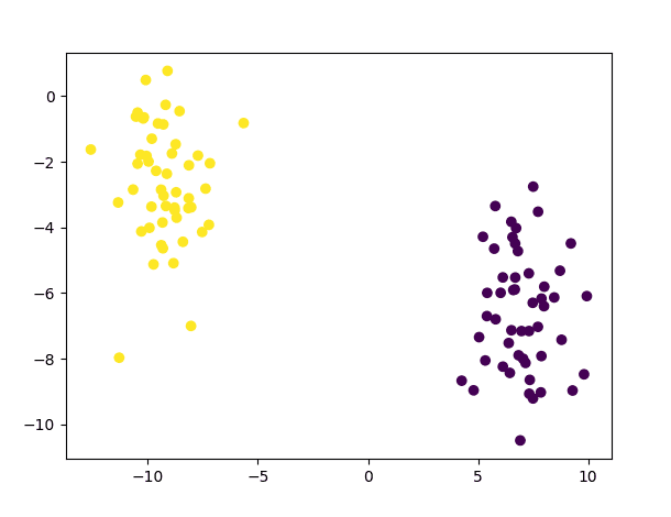
We may see that the class predictions produced by the normal Bayes classifier trained on this simple dataset are correct:

Scatter Plot of Predictions Generated for the Test Samples

Image Segmentation Using a Normal Bayes Classifier

Among their many applications, Bayes classifiers have been frequently used for skin segmentation, which separates skin pixels from non-skin pixels in an image.

We can adapt the code above for segmenting skin pixels in images. For this purpose, we will use the Skin Segmentation dataset, consisting of 50,859 skin samples and 194,198 non-skin samples, to train the normal Bayes classifier. The dataset presents the pixel values in BGR order and their corresponding class label.

After loading the dataset, we shall convert the BGR pixel values into HSV (denoting Hue, Saturation, and Value) and then use the hue values to train a normal Bayes classifier. Hue is often preferred over RGB in image segmentation tasks because it represents the true color without modification and is less affected by lighting variations than RGB. In the HSV color model, the hue values are arranged radially and span between 0 and 360 degrees:

from cv2 import ml,
from numpy import loadtxt, float32
from matplotlib.colors import rgb_to_hsv

# Load data from text file
data = loadtxt("Data/Skin_NonSkin.txt", dtype=int)

# Select the BGR values from the loaded data
BGR = data[:, :3]

# Convert to RGB by swapping the array columns
RGB = BGR.copy()
RGB[:, [2, 0]] = RGB[:, [0, 2]]

# Convert RGB values to HSV
HSV = rgb_to_hsv(RGB.reshape(RGB.shape[0], -1, 3) / 255)
HSV = HSV.reshape(RGB.shape[0], 3)

# Select only the hue values
hue = HSV[:, 0] * 360

# Select the labels from the loaded data
labels = data[:, -1]

# Create a new Normal Bayes Classifier
norm_bayes = ml.NormalBayesClassifier_create()

# Train the classifier on the hue values
norm_bayes.train(hue.astype(float32), ml.ROW_SAMPLE, labels)

from cv2 import ml,

from numpy import loadtxt, float32

from matplotlib.colors import rgb_to_hsv

# Load data from text file

data = loadtxt("Data/Skin_NonSkin.txt", dtype=int)

# Select the BGR values from the loaded data

BGR = data[:, :3]

# Convert to RGB by swapping the array columns

RGB = BGR.copy()

RGB[:, [2, 0]] = RGB[:, [0, 2]]

# Convert RGB values to HSV

HSV = rgb_to_hsv(RGB.reshape(RGB.shape[0], -1, 3) / 255)

HSV = HSV.reshape(RGB.shape[0], 3)

# Select only the hue values

hue = HSV[:, 0] * 360

# Select the labels from the loaded data

labels = data[:, -1]

# Create a new Normal Bayes Classifier

norm_bayes = ml.NormalBayesClassifier_create()

# Train the classifier on the hue values

norm_bayes.train(hue.astype(float32), ml.ROW_SAMPLE, labels)

Note 1: The OpenCV library provides the cvtColor method to convert between color spaces, as seen in this tutorial, but the cvtColor method expects the source image in its original shape as an input. The rgb_to_hsv method in Matplotlib, on the other hand, accepts a NumPy array in the form of (…, 3) as input, where the array values are expected to be normalized within the range of 0 to 1. We are using the latter here since our training data consists of individual pixels, which are not structured in the usual form of a three-channel image.

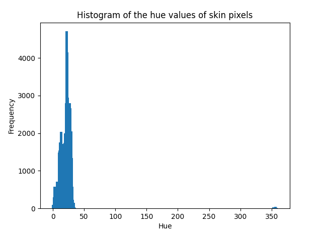
Note 2: The normal Bayes classifier assumes that the data to be modeled follows a Gaussian distribution. While this is not a strict requirement, the classifier’s performance may degrade if the data is distributed otherwise. We may check the distribution of the data we are working with by plotting its histogram. If we take the hue values of the skin pixels as an example, we find that a Gaussian curve can describe their distribution:

from numpy import histogram
from matplotlib.pyplot import bar, title, xlabel, ylabel, show

# Choose the skin-labelled hue values
skin = x[labels == 1]

# Compute their histogram
hist, bin_edges = histogram(skin, range=[0, 360], bins=360)

# Display the computed histogram
bar(bin_edges[:-1], hist, width=4)
xlabel('Hue')
ylabel('Frequency')
title('Histogram of the hue values of skin pixels')
show()

from numpy import histogram

from matplotlib.pyplot import bar, title, xlabel, ylabel, show

# Choose the skin-labelled hue values

skin = x[labels == 1]

# Compute their histogram

hist, bin_edges = histogram(skin, range=[0, 360], bins=360)

# Display the computed histogram

bar(bin_edges[:-1], hist, width=4)

xlabel('Hue')

ylabel('Frequency')

title('Histogram of the hue values of skin pixels')

show()

Checking the Distribution of the Data

Once the normal Bayes classifier has been trained, we may test it out on an image (let’s consider this example image for testing):

from cv2 import imread
from matplotlib.pyplot import show, imshow

# Load a test image
face_img = imread("Images/face.jpg")

# Reshape the image into a three-column array
face_BGR = face_img.reshape(-1, 3)

# Convert to RGB by swapping the array columns
face_RGB = face_BGR.copy()
face_RGB[:, [2, 0]] = face_RGB[:, [0, 2]]

# Convert from RGB to HSV
face_HSV = rgb_to_hsv(face_RGB.reshape(face_RGB.shape[0], -1, 3) / 255)
face_HSV = face_HSV.reshape(face_RGB.shape[0], 3)

# Select only the hue values
face_hue = face_HSV[:, 0] * 360

# Display the hue image
imshow(face_hue.reshape(face_img.shape[0], face_img.shape[1]))
show()

# Generate a prediction from the trained classifier
ret, labels_pred, output_probs = norm_bayes.predictProb(face_hue.astype(float32))

# Reshape array into the input image size and choose the skin-labelled pixels
skin_mask = labels_pred.reshape(face_img.shape[0], face_img.shape[1], 1) == 1

# Display the segmented image
imshow(skin_mask, cmap='gray')
show()

from cv2 import imread

from matplotlib.pyplot import show, imshow

# Load a test image

face_img = imread("Images/face.jpg")

# Reshape the image into a three-column array

face_BGR = face_img.reshape(-1, 3)

# Convert to RGB by swapping the array columns

face_RGB = face_BGR.copy()

face_RGB[:, [2, 0]] = face_RGB[:, [0, 2]]

# Convert from RGB to HSV

face_HSV = rgb_to_hsv(face_RGB.reshape(face_RGB.shape[0], -1, 3) / 255)

face_HSV = face_HSV.reshape(face_RGB.shape[0], 3)

# Select only the hue values

face_hue = face_HSV[:, 0] * 360

# Display the hue image

imshow(face_hue.reshape(face_img.shape[0], face_img.shape[1]))

show()

# Generate a prediction from the trained classifier

ret, labels_pred, output_probs = norm_bayes.predictProb(face_hue.astype(float32))

# Reshape array into the input image size and choose the skin-labelled pixels

skin_mask = labels_pred.reshape(face_img.shape[0], face_img.shape[1], 1) == 1

# Display the segmented image

imshow(skin_mask, cmap='gray')

show()

The resulting segmented mask displays the pixels labeled as belonging to the skin (with a class label equal to 1).

By qualitatively analyzing the result, we may see that most of the skin pixels have been correctly labeled as such. We may also see that some hair strands (hence, non-skin pixels) have been incorrectly labeled as belonging to skin. If we had to look at their hue values, we might notice that these are very similar to those belonging to skin regions, hence the mislabelling. Furthermore, we may also notice the effectiveness of using the hue values, which remain relatively constant in regions of the face that otherwise appear illuminated or in shadow in the original RGB image:

Original Image (Left); Hue Values (Middle); Segmented Skin Pixels (Right)

Can you think of more tests to try out with a normal Bayes classifier?

Summary

In this tutorial, you learned how to apply OpenCV’s normal Bayes algorithm, first on a custom two-dimensional dataset and subsequently for segmenting an image.

Specifically, you learned:

Several of the most important points in applying the Bayes theorem to machine learning.
How to use the normal Bayes algorithm on a custom dataset in OpenCV.
How to use the normal Bayes algorithm to segment an image in OpenCV.

Do you have any questions?

Ask your questions in the comments below, and I will do my best to answer.

Get Started on Machine Learning in OpenCV!

Learn how to use machine learning techniques in image processing projects

...using OpenCV in advanced ways and work beyond pixels

Discover how in my new Ebook:
Machine Learing in OpenCV

It provides self-study tutorials with all working code in Python to turn you from a novice to expert. It equips you with
logistic regression, random forest, SVM, k-means clustering, neural networks, and much more...all using the machine learning module in OpenCV

Kick-start your deep learning journey with hands-on exercises

See What's Inside

Navigation

Normal Bayes Classifier for Image Segmentation Using OpenCV

Tutorial Overview

Reminder of the Bayes Theorem As Applied to Machine Learning

Discovering Bayes Classification in OpenCV

Want to Get Started With Machine Learning with OpenCV?

Image Segmentation Using a Normal Bayes Classifier

Further Reading

Books

Summary

Get Started on Machine Learning in OpenCV!

Learn how to use machine learning techniques in image processing projects

Kick-start your deep learning journey with hands-on exercises

More On This Topic

No comments yet.

Leave a Reply Click here to cancel reply.