The k-means clustering algorithm is an unsupervised machine learning technique that seeks to group similar data into distinct clusters to uncover patterns in the data that may not be apparent to the naked eye.
It is possibly the most widely known algorithm for data clustering and is implemented in the OpenCV library.
In this tutorial, you will learn how to apply OpenCV’s k-means clustering algorithm for color quantization of images.
After completing this tutorial, you will know:
What data clustering is within the context of machine learning.
Applying the k-means clustering algorithm in OpenCV to a simple two-dimensional dataset containing distinct data clusters.
How to apply the k-means clustering algorithm in OpenCV for color quantization of images.
Kick-start your project with my book Machine Learning in OpenCV. It provides self-study tutorials with working code.
Let’s get started.
K-Means Clustering for Color Quantization Using OpenCV Photo by Billy Huynh, some rights reserved.
Tutorial Overview
This tutorial is divided into three parts; they are:
Clustering as an Unsupervised Machine Learning Task
Discovering k-Means Clustering in OpenCV
Color Quantization Using k-Means
Clustering as an Unsupervised Machine Learning Task
Cluster analysis is an unsupervised learning technique.
It involves automatically grouping data into distinct groups (or clusters), where the data within each cluster are similar but different from those in the other clusters. It aims to uncover patterns in the data that may not be apparent before clustering.
There are many different clustering algorithms, as explained in this tutorial, with k-means clustering being one of the most widely known.
The k-means clustering algorithm takes unlabelled data points. It seeks to assign them to kclusters, where each data point belongs to the cluster with the nearest cluster center, and the center of each cluster is taken as the mean of the data points that belong to it. The algorithm requires that the user provide the value of k as an input; hence, this value needs to be known a priori or tuned according to the data.
Discovering k-Means Clustering in OpenCV
Let’s first consider applying k-means clustering to a simple two-dimensional dataset containing distinct data clusters before moving on to more complex tasks.
For this purpose, we shall be generating a dataset consisting of 100 data points (specified by n_samples), which are equally divided into 5 Gaussian clusters (identified by centers) having a standard deviation set to 1.5 (determined by cluster_std). To be able to replicate the results, let’s also define a value for random_state, which we’re going to set to 10:
Python
1
2
3
4
5
6
# Generating a dataset of 2D data points and their ground truth labels
The code above should generate the following plot of data points:
Scatter Plot of Dataset Consisting of 5 Gaussian Clusters
Want to Get Started With Machine Learning with OpenCV?
Take my free email crash course now (with sample code).
Click to sign-up and also get a free PDF Ebook version of the course.
If we look at this plot, we may already be able to visually distinguish one cluster from another, which means that this should be a sufficiently straightforward task for the k-means clustering algorithm.
In OpenCV, the k-means algorithm is not part of the ml module but can be called directly. To be able to use it, we need to specify values for its input arguments as follows:
The input, unlabelled data.
The number, K, of required clusters.
The termination criteria, TERM_CRITERIA_EPS and TERM_CRITERIA_MAX_ITER, defining the desired accuracy and the maximum number of iterations, respectively, which, when reached, the algorithm iteration should stop.
The number of attempts, denoting the number of times the algorithm will be executed with different initial labeling to find the best cluster compactness.
How the cluster centers will be initialized, whether random, user-supplied, or through a center initialization method such as kmeans++, as specified by the parameter flags.
The k-means clustering algorithm in OpenCV returns:
The compactness of each cluster, computed as the sum of the squared distance of each data point to its corresponding cluster center. A smaller compactness value indicates that the data points are distributed closer to their corresponding cluster center and, hence, the cluster is more compact.
The predicted cluster labels y_pred, associate each input data point with its corresponding cluster.
The centers coordinates of each cluster of data points.
Let’s now apply the k-means clustering algorithm to the dataset generated earlier. Note that we are type-casting the input data to float32, as expected by the kmeans() function in OpenCV:
# Plot the data clusters, each having a different color, together with the corresponding cluster centers
scatter(x[:,0],x[:,1],c=y_pred)
scatter(centers[:,0],centers[:,1],c='red')
show()
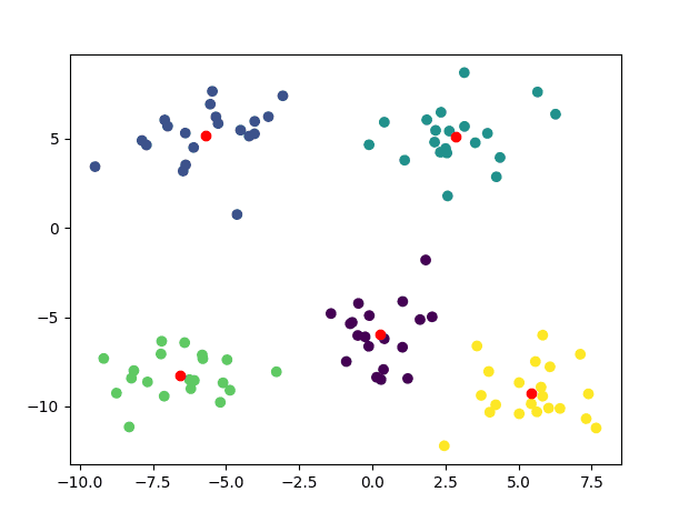
The code above generates the following plot, where each data point is now colored according to its assigned cluster, and the cluster centers are marked in red:
Scatter Plot of Dataset With Clusters Identified Using k-Means Clustering
# Plot the data clusters, each having a different colour, together with the corresponding cluster centers
scatter(x[:,0],x[:,1],c=y_pred)
scatter(centers[:,0],centers[:,1],c='red')
show()
Color Quantization Using k-Means
One of the applications for k-means clustering is the color quantization of images.
Color quantization refers to the process of reducing the number of distinct colors that are used in the representation of an image.
Color quantization is critical for displaying images with many colors on devices that can only display a limited number of colors, usually due to memory limitations, and enables efficient compression of certain types of images.
In this case, the data points that we will provide to the k-means clustering algorithm are the RGB values of each image pixel. As we shall be seeing, we will provide these values in the form of an $M \times 3$ array, where $M$ denotes the number of pixels in the image.
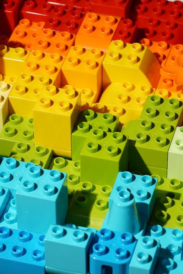
Let’s try out the k-means clustering algorithm on this image, which I have named bricks.jpg:
The dominant colors that stand out in this image are red, orange, yellow, green, and blue. However, many shadows and glints introduce additional shades and colors to the dominant ones.
We’ll start by first reading the image using OpenCV’s imread function.
Remember that OpenCV loads this image in BGR rather than RGB order. There is no need to convert it to RGB before feeding it to the k-means clustering algorithm because the latter will still group similar colors no matter in which order the pixel values are specified. However, since we are making use of Matplotlib to display the images, we’ll convert it to RGB so that we may display the quantized result correctly later on:
Python
1
2
3
4
5
# Read image
img=imread('Images/bricks.jpg')
# Convert it from BGR to RGB
img_RGB=cvtColor(img,COLOR_BGR2RGB)
As we have mentioned earlier, the next step involves reshaping the image to an $M \times 3$ array, and we may then proceed to apply k-means clustering to the resulting array values using several clusters that correspond to the number of dominant colors we have mentioned above.
In the code snippet below, I have also included a line that prints out the number of unique RGB pixel values from the total number of pixels in the image. We find that we have 338,742 unique RGB values out of 14,155,776 pixels, which is substantial:
Python
1
2
3
4
5
6
7
8
9
10
11
# Reshape image to an Mx3 array
img_data=img_RGB.reshape(-1,3)
# Find the number of unique RGB values
print(len(unique(img_data,axis=0)),'unique RGB values out of',img_data.shape[0],'pixels')
At this point, we shall proceed to apply the actual RGB values of the cluster centers to the predicted pixel labels and reshape the resulting array to the shape of the original image before displaying it:
Python
1
2
3
4
5
6
7
8
9
10
11
12
# Apply the RGB values of the cluster centers to all pixel labels
colours=centers[labels].reshape(-1,3)
# Find the number of unique RGB values
print(len(unique(colours,axis=0)),'unique RGB values out of',img_data.shape[0],'pixels')
# Reshape array to the original image shape
img_colours=colours.reshape(img_RGB.shape)
# Display the quantized image
imshow(img_colours.astype(uint8))
show()
Printing again the number of unique RGB values in the quantized image, we find that these have now lessened to the number of clusters that we had specified to the k-means algorithm:
Python
1
5 unique RGB values out of 14155776 pixels
If we look at the color quantized image, we find that the pixels belonging to the yellow and orange bricks have been grouped into the same cluster, possibly due to the similarity of their RGB values. In contrast, one of the clusters aggregates pixels belonging to regions of shadow:
Color Quantized Image Using k-Means Clustering with 5 Clusters
Now try changing the value specifying the number of clusters for the k-means clustering algorithm and investigate its effect on the quantization result.
It provides self-study tutorials with all working code in Python to turn you from a novice to expert. It equips you with logistic regression, random forest, SVM, k-means clustering, neural networks,
and much more...all using the machine learning module in OpenCV
Kick-start your deep learning journey with hands-on exercises
Does K-Means Clustering with only one center equal averaging all pixel values?
For example if I want to calculate the main color of a car, should I average all of the car’s image’s pixel values to get the main color or should I do a K-Means clustering with a cluster of size one on all of the pixels?
Hi Mohammad. IMHO, if you see a car in an image, it is because there is the car AND was is not the car, let’s call this a background. Necessarily, the background as a different color than the car since otherwise the car would be invisible. So try a k-means with at least 2 color so that one of the group can indicate the pixels of the car. Then you can average the colors of these pixels.


 From Scratch With Python")


Thanks for the great articles.
Just one question:
Does K-Means Clustering with only one center equal averaging all pixel values?
For example if I want to calculate the main color of a car, should I average all of the car’s image’s pixel values to get the main color or should I do a K-Means clustering with a cluster of size one on all of the pixels?
Thanks
Hi Mohammad…Your approach is reasonable! Proceed with your model and let us know what you find!
Jason, you are the best. This is a wonderful article. I enjoyed it.
Thank you for your feedback and support David! We greatly apprecite it! Let us know if you ever have any questions regarding our content.
Hi Mohammad. IMHO, if you see a car in an image, it is because there is the car AND was is not the car, let’s call this a background. Necessarily, the background as a different color than the car since otherwise the car would be invisible. So try a k-means with at least 2 color so that one of the group can indicate the pixels of the car. Then you can average the colors of these pixels.