In a previous tutorial, we explored using the k-means clustering algorithm as an unsupervised machine learning technique that seeks to group similar data into distinct clusters to uncover patterns in the data.
So far, we have seen how to apply the k-means clustering algorithm to a simple two-dimensional dataset containing distinct clusters and the problem of image color quantization.
In this tutorial, you will learn how to apply OpenCV’s k-means clustering algorithm for image classification.
After completing this tutorial, you will know:
- Why k-means clustering can be applied to image classification.
- Applying the k-means clustering algorithm to the digit dataset in OpenCV for image classification.
- How to reduce the digit variations due to skew to improve the accuracy of the k-means clustering algorithm for image classification.
Kick-start your project with my book Machine Learning in OpenCV. It provides self-study tutorials with working code.
Let’s get started.

K-Means Clustering for Image Classification Using OpenCV
Photo by Jeremy Thomas, some rights reserved.
Tutorial Overview
This tutorial is divided into two parts; they are:
- Recap of k-Means Clustering as an Unsupervised Machine Learning Technique
- Applying k-Means Clustering to Image Classification
Recap of k-Means Clustering as an Unsupervised Machine Learning Technique
In a previous tutorial, we have been introduced to k-means clustering as an unsupervised learning technique.
We have seen that this technique involves automatically grouping data into distinct groups (or clusters), where the data within each cluster are similar to one another but different from those in the other clusters. It aims to uncover patterns in the data that may not be apparent before clustering.
We have applied the k-means clustering algorithm to a simple two-dimensional dataset containing five clusters to label the data points belonging to each cluster accordingly, and subsequently to the task of color quantization where we have used this algorithm to reduce the number of distinct colors representing an image.
In this tutorial, we shall again exploit the strength of k-means clustering in uncovering hidden structures in the data by applying it to the image classification task.
For such a task, we will be employing the OpenCV digits dataset introduced in a previous tutorial, where we will aim to try to group images of similar handwritten digits in an unsupervised manner (i.e., without using the ground truth label information).
Applying k-Means Clustering to Image Classification
We’ll first need to load the OpenCV digits image, divide it into its many sub-images that feature handwritten digits from 0 to 9, and create their corresponding ground truth labels that will enable us to quantify the performance of the k-means clustering algorithm later on:
|
1 2 3 4 5 |
# Load the digits image and divide it into sub-images img, sub_imgs = split_images('Images/digits.png', 20) # Create the ground truth labels imgs, labels_true, _, _ = split_data(20, sub_imgs, 1.0) |
The returned imgs array contains 5,000 sub-images, organized row-wise in the form of flattened one-dimensional vectors, each comprising 400 pixels:
|
1 2 |
# Check the shape of the 'imgs' array print(imgs.shape) |
|
1 |
(5000, 400) |
The k-means algorithm can subsequently be provided with input arguments that are equivalent to those that we have used for our color quantization example, with the only exception being that we’ll need to pass the imgs array as the input data, and that we shall be setting the value of K clusters to 10 (i.e., the number of digits that we have available):
|
1 2 3 4 5 |
# Specify the algorithm's termination criteria criteria = (TERM_CRITERIA_MAX_ITER + TERM_CRITERIA_EPS, 10, 1.0) # Run the k-means clustering algorithm on the image data compactness, clusters, centers = kmeans(data=imgs.astype(float32), K=10, bestLabels=None, criteria=criteria, attempts=10, flags=KMEANS_RANDOM_CENTERS) |
The kmeans function returns a centers array, which should contain a representative image for each cluster. The returned centers array is of shape 10$\times$400, which means that we’ll first need to reshape it back to 20$\times$20 pixel images before proceeding to visual them:
|
1 2 3 4 5 6 7 8 9 10 |
# Reshape array into 20x20 images imgs_centers = centers.reshape(-1, 20, 20) # Visualise the cluster centers fig, ax = subplots(2, 5) for i, center in zip(ax.flat, imgs_centers): i.imshow(center) show() |
The representative images of the cluster centers are as follows:
It is remarkable that the cluster centers generated by the k-means algorithm indeed resemble the handwritten digits contained in the OpenCV digits dataset.
You may also notice that the order of the cluster centers does not necessarily follow the order of the digits from 0 to 9. This is because the k-means algorithm can cluster similar data together but has no notion of its order. However, it also creates a problem when comparing the predicted labels with the ground truth ones. This is because the ground truth labels have been generated to correspond to the digit numbers featured inside the images. However, the cluster labels generated by the k-means algorithm do not necessarily follow the same convention. To solve this problem, we need to re-order the cluster labels:
|
1 2 3 4 5 6 7 8 9 |
# Found cluster labels labels = array([2, 0, 7, 5, 1, 4, 6, 9, 3, 8]) labels_pred = zeros(labels_true.shape, dtype='int') # Re-order the cluster labels for i in range(10): mask = clusters.ravel() == i labels_pred[mask] = labels[i] |
Now we’re ready to calculate the accuracy of the algorithm, by finding the percentage of predicted labels that correspond to the ground truth:
|
1 2 3 4 5 |
# Calculate the algorithm's accuracy accuracy = (sum(labels_true == labels_pred) / labels_true.size) * 100 # Print the accuracy print("Accuracy: {0:.2f}%".format(accuracy[0])) |
|
1 |
Accuracy: 54.80% |
The complete code listing up to this point is as follows:
|
1 2 3 4 5 6 7 8 9 10 11 12 13 14 15 16 17 18 19 20 21 22 23 24 25 26 27 28 29 30 31 32 33 34 35 36 37 38 39 40 41 42 43 |
from cv2 import kmeans, TERM_CRITERIA_MAX_ITER, TERM_CRITERIA_EPS, KMEANS_RANDOM_CENTERS from numpy import float32, array, zeros from matplotlib.pyplot import show, imshow, subplots from digits_dataset import split_images, split_data # Load the digits image and divide it into sub-images img, sub_imgs = split_images('Images/digits.png', 20) # Create the ground truth labels imgs, labels_true, _, _ = split_data(20, sub_imgs, 1.0) # Check the shape of the 'imgs' array print(imgs.shape) # Specify the algorithm's termination criteria criteria = (TERM_CRITERIA_MAX_ITER + TERM_CRITERIA_EPS, 10, 1.0) # Run the k-means clustering algorithm on the image data compactness, clusters, centers = kmeans(data=imgs.astype(float32), K=10, bestLabels=None, criteria=criteria, attempts=10, flags=KMEANS_RANDOM_CENTERS) # Reshape array into 20x20 images imgs_centers = centers.reshape(-1, 20, 20) # Visualise the cluster centers fig, ax = subplots(2, 5) for i, center in zip(ax.flat, imgs_centers): i.imshow(center) show() # Cluster labels labels = array([2, 0, 7, 5, 1, 4, 6, 9, 3, 8]) labels_pred = zeros(labels_true.shape, dtype='int') # Re-order the cluster labels for i in range(10): mask = clusters.ravel() == i labels_pred[mask] = labels[i] # Calculate the algorithm's accuracy accuracy = (sum(labels_true == labels_pred) / labels_true.size) * 100 |
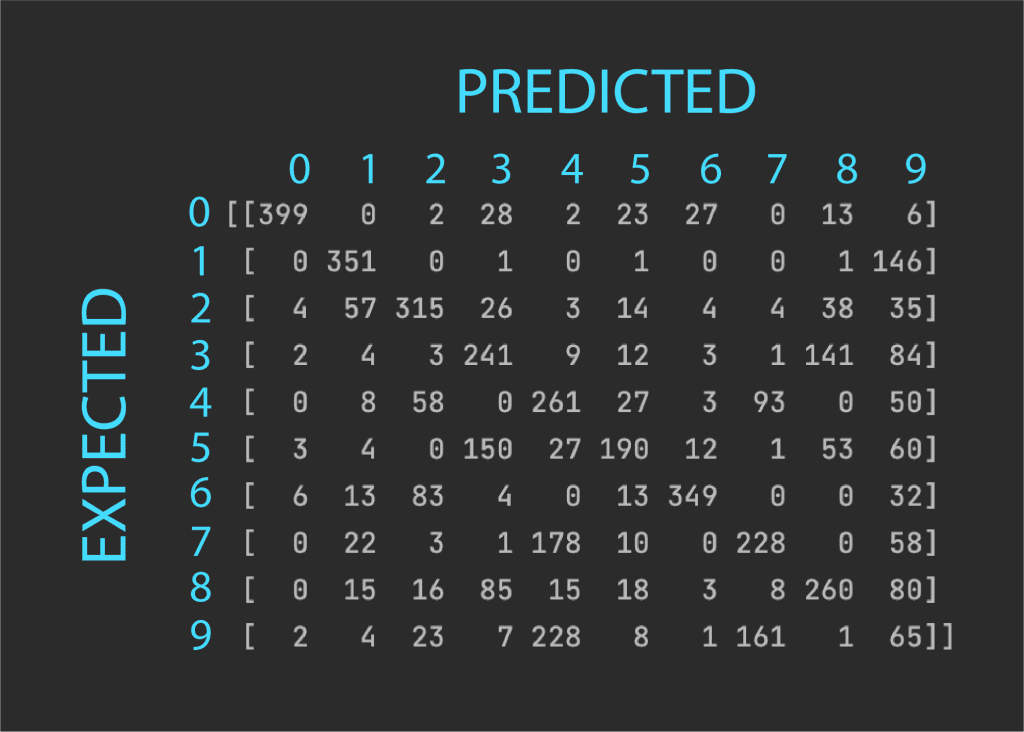
Now, let’s print out the confusion matrix to gain a deeper insight into which digits have been mistaken for one another:
|
1 2 3 4 |
from sklearn.metrics import confusion_matrix # Print confusion matrix print(confusion_matrix(labels_true, labels_pred)) |
|
1 2 3 4 5 6 7 8 9 10 |
[[399 0 2 28 2 23 27 0 13 6] [ 0 351 0 1 0 1 0 0 1 146] [ 4 57 315 26 3 14 4 4 38 35] [ 2 4 3 241 9 12 3 1 141 84] [ 0 8 58 0 261 27 3 93 0 50] [ 3 4 0 150 27 190 12 1 53 60] [ 6 13 83 4 0 13 349 0 0 32] [ 0 22 3 1 178 10 0 228 0 58] [ 0 15 16 85 15 18 3 8 260 80] [ 2 4 23 7 228 8 1 161 1 65]] |
The confusion matrix needs to be interpreted as follows:
The values on the diagonal indicate the number of correctly predicted digits, whereas the off-diagonal values indicate the misclassifications per digit. We may see that the best performing digit is 0, with the highest diagonal value and very few misclassifications. The worst performing digit is 9 since this has the highest number of misclassifications with many other digits, mostly with 4. We may also see that 7 has been mostly mistaken with 4, while 8 has been mostly mistaken with 3.
These results do not necessarily come as a surprise because, if we had to look at the digits in the dataset, we might see that the curves and skew of several different digits cause them to resemble each other. To investigate the effect of reducing the digit variations, let’s introduce a function, deskew_image(), that applies an affine transformation to an image based on a measure of skew calculated from the image moments:
|
1 2 3 4 5 6 7 8 9 10 11 12 13 14 15 16 17 18 19 20 21 22 23 24 25 26 27 28 29 30 31 32 33 34 35 36 37 38 39 40 41 42 43 44 45 46 47 48 49 50 51 52 53 54 55 56 57 58 59 60 61 62 63 64 65 66 67 68 69 70 71 72 73 74 75 76 77 78 79 80 81 |
from cv2 import (kmeans, TERM_CRITERIA_MAX_ITER, TERM_CRITERIA_EPS, KMEANS_RANDOM_CENTERS, moments, warpAffine, INTER_CUBIC, WARP_INVERSE_MAP) from numpy import float32, array, zeros from matplotlib.pyplot import show, imshow, subplots from digits_dataset import split_images, split_data from sklearn.metrics import confusion_matrix # Load the digits image and divide it into sub-images img, sub_imgs = split_images('Images/digits.png', 20) # Create the ground truth labels imgs, labels_true, _, _ = split_data(20, sub_imgs, 1.0) # De-skew all dataset images imgs_deskewed = zeros(imgs.shape) for i in range(imgs_deskewed.shape[0]): new = deskew_image(imgs[i, :].reshape(20, 20)) imgs_deskewed[i, :] = new.reshape(1, -1) # Specify the algorithm's termination criteria criteria = (TERM_CRITERIA_MAX_ITER + TERM_CRITERIA_EPS, 10, 1.0) # Run the k-means clustering algorithm on the de-skewed image data compactness, clusters, centers = kmeans(data=imgs_deskewed.astype(float32), K=10, bestLabels=None, criteria=criteria, attempts=10, flags=KMEANS_RANDOM_CENTERS) # Reshape array into 20x20 images imgs_centers = centers.reshape(-1, 20, 20) # Visualise the cluster centers fig, ax = subplots(2, 5) for i, center in zip(ax.flat, imgs_centers): i.imshow(center) show() # Cluster labels labels = array([9, 5, 6, 4, 2, 3, 7, 8, 1, 0]) labels_pred = zeros(labels_true.shape, dtype='int') # Re-order the cluster labels for i in range(10): mask = clusters.ravel() == i labels_pred[mask] = labels[i] # Calculate the algorithm's accuracy accuracy = (sum(labels_true == labels_pred) / labels_true.size) * 100 # Print the accuracy print("Accuracy: {0:.2f}%".format(accuracy[0])) # Print confusion matrix print(confusion_matrix(labels_true, labels_pred)) def deskew_image(img): # Calculate the image moments img_moments = moments(img) # Moment m02 indicates how much the pixel intensities are spread out along the vertical axis if abs(img_moments['mu02']) > 1e-2: # Calculate the image skew img_skew = (img_moments['mu11'] / img_moments['mu02']) # Generate the transformation matrix # (We are here tweaking slightly the approximation of vertical translation due to skew by making use of a # scaling factor of 0.6, because we empirically found that this value worked better for this application) m = float32([[1, img_skew, -0.6 * img.shape[0] * img_skew], [0, 1, 0]]) # Apply the transformation matrix to the image img_deskew = warpAffine(src=img, M=m, dsize=img.shape, flags=INTER_CUBIC | WARP_INVERSE_MAP) else: # If the vertical spread of pixel intensities is small, return a copy of the original image img_deskew = img.copy() return img_deskew |
|
1 2 3 4 5 6 7 8 9 10 11 12 |
Accuracy: 70.92% [[400 1 5 1 2 58 27 1 1 4] [ 0 490 1 1 0 1 2 0 1 4] [ 5 27 379 28 10 2 3 4 30 12] [ 1 27 7 360 7 44 2 9 31 12] [ 1 29 3 0 225 0 13 1 0 228] [ 5 12 1 14 24 270 11 0 7 156] [ 8 40 6 0 6 8 431 0 0 1] [ 0 39 2 0 48 0 0 377 4 30] [ 2 32 3 21 8 77 2 0 332 23] [ 5 13 1 5 158 5 2 28 1 282]] |
The de-skewing function has the following effect on some of the digits:

The First Column Depicts the Original Dataset Images, While the Second Column Shows Images Corrected for Skew
Remarkably, the accuracy rises to 70.92% when the skew of the digits is reduced, while the cluster centers become more representative of the digits in the dataset:
This result shows that skew was a highly contributing factor to the loss of accuracy that we experienced without its correction.
Can you think of any other pre-processing steps you may introduce to improve the accuracy?
Want to Get Started With Machine Learning with OpenCV?
Take my free email crash course now (with sample code).
Click to sign-up and also get a free PDF Ebook version of the course.
Further Reading
This section provides more resources on the topic if you want to go deeper.
Books
- Machine Learning for OpenCV, 2017.
- Mastering OpenCV 4 with Python, 2019.
Websites
- 10 Clustering Algorithms With Python, https://machinelearningmastery.com/clustering-algorithms-with-python/
- K-Means Clustering in OpenCV, https://docs.opencv.org/3.4/d1/d5c/tutorial_py_kmeans_opencv.html
- k-means clustering, https://en.wikipedia.org/wiki/K-means_clustering
Summary
In this tutorial, you learned how to apply OpenCV’s k-means clustering algorithm for image classification.
Specifically, you learned:
- Why k-means clustering can be applied to image classification.
- Applying the k-means clustering algorithm to the digit dataset in OpenCV for image classification.
- How to reduce the digit variations due to skew to improve the accuracy of the k-means clustering algorithm for image classification.
Do you have any questions?
Ask your questions in the comments below, and I will do my best to answer.







For such a task, we will be employing the OpenCV digits dataset introduced in a “previous tutorial”
The link embedded within ‘previous tutorial’ is invalid.
Thank you for your feedback shincheng!