In a previous tutorial, we explored using the Support Vector Machine algorithm as one of the most popular supervised machine learning techniques implemented in the OpenCV library.
So far, we have seen how to apply Support Vector Machines to a custom dataset that we have generated, consisting of two-dimensional points gathered into two classes.
In this tutorial, you will learn how to apply OpenCV’s Support Vector Machine algorithm to solve image classification and detection problems.
After completing this tutorial, you will know:
- Several of the most important characteristics of Support Vector Machines.
- How to apply Support Vector Machines to the problems of image classification and detection.
Kick-start your project with my book Machine Learning in OpenCV. It provides self-study tutorials with working code.
Let’s get started.

Support Vector Machines for Image Classification and Detection Using OpenCV
Photo by Patrick Ryan, some rights reserved.
Tutorial Overview
This tutorial is divided into three parts; they are:
- Recap of How Support Vector Machines Work
- Applying the SVM Algorithm to Image Classification
- Using the SVM Algorithm for Image Detection
Recap of How Support Vector Machines Work
In a previous tutorial, we were introduced to using the Support Vector Machine (SVM) algorithm in the OpenCV library. So far, we have applied it to a custom dataset that we have generated, consisting of two-dimensional points gathered into two classes.
We have seen that SVMs seek to separate data points into classes by computing a decision boundary that maximizes the margin to the closest data points from each class, called the support vectors. The constraint of maximizing the margin can be relaxed by tuning a parameter called C, which controls the trade-off between maximizing the margin and reducing the misclassifications on the training data.
The SVM algorithm may use different kernel functions, depending on whether the input data is linearly separable. In the case of non-linearly separable data, a non-linear kernel may be used to transform the data to a higher-dimensional space in which it becomes linearly separable. This is analogous to the SVM finding a non-linear decision boundary in the original input space.
Applying the SVM Algorithm to Image Classification
We will use the digits dataset in OpenCV for this task, although the code we will develop may also be used with other datasets.
Want to Get Started With Machine Learning with OpenCV?
Take my free email crash course now (with sample code).
Click to sign-up and also get a free PDF Ebook version of the course.
Our first step is to load the OpenCV digits image, divide it into its many sub-images that feature handwritten digits from 0 to 9, and create their corresponding ground truth labels that will enable us to quantify the accuracy of the trained SVM classifier later. For this particular example, we will allocate 80% of the dataset images to the training set and the remaining 20% of the images to the testing set:
|
1 2 3 4 5 |
# Load the digits image img, sub_imgs = split_images('Images/digits.png', 20) # Obtain training and testing datasets from the digits image digits_train_imgs, digits_train_labels, digits_test_imgs, digits_test_labels = split_data(20, sub_imgs, 0.8) |
Our next step is to create an SVM in OpenCV that uses an RBF kernel. As we have done in our previous tutorial, we must set several parameter values related to the SVM type and the kernel function. We shall also include the termination criteria to stop the iterative process of the SVM optimization problem:
|
1 2 3 4 5 6 7 8 9 |
# Create a new SVM svm_digits = ml.SVM_create() # Set the SVM kernel to RBF svm_digits.setKernel(ml.SVM_RBF) svm_digits.setType(ml.SVM_C_SVC) svm_digits.setGamma(0.5) svm_digits.setC(12) svm_digits.setTermCriteria((TERM_CRITERIA_MAX_ITER + TERM_CRITERIA_EPS, 100, 1e-6)) |
Rather than training and testing the SVM on the raw image data, we will first convert each image into its HOG descriptors, as explained in this tutorial. The HOG technique aims for a more compact representation of an image by exploiting its local shape and appearance. Training a classifier on HOG descriptors can potentially increase its discriminative power in distinguishing between different classes while at the same time reducing the computational expense of processing the data:
|
1 2 3 |
# Converting the image data into HOG descriptors digits_train_hog = hog_descriptors(digits_train_imgs) digits_test_hog = hog_descriptors(digits_test_imgs) |
We may finally train the SVM on the HOG descriptors and proceed to predict labels for the testing data, based on which we may compute the classifier’s accuracy:
|
1 2 3 4 5 6 |
# Predict labels for the testing data _, digits_test_pred = svm_digits.predict(digits_test_hog.astype(float32)) # Compute and print the achieved accuracy accuracy_digits = (sum(digits_test_pred.astype(int) == digits_test_labels) / digits_test_labels.size) * 100 print('Accuracy:', accuracy_digits[0], '%') |
|
1 |
Accuracy: 97.1 % |
For this particular example, the values for C and gamma are being set empirically. However, it is suggested that a tuning technique, such as the grid search algorithm, is employed to investigate whether a better combination of hyperparameters can push the classifier’s accuracy even higher.
The complete code listing is as follows:
|
1 2 3 4 5 6 7 8 9 10 11 12 13 14 15 16 17 18 19 20 21 22 23 24 25 26 27 28 29 30 31 32 33 34 35 |
from cv2 import ml, TERM_CRITERIA_MAX_ITER, TERM_CRITERIA_EPS from numpy import float32 from digits_dataset import split_images, split_data from feature_extraction import hog_descriptors # Load the digits image img, sub_imgs = split_images('Images/digits.png', 20) # Obtain training and testing datasets from the digits image digits_train_imgs, digits_train_labels, digits_test_imgs, digits_test_labels = split_data(20, sub_imgs, 0.8) # Create a new SVM svm_digits = ml.SVM_create() # Set the SVM kernel to RBF svm_digits.setKernel(ml.SVM_RBF) svm_digits.setType(ml.SVM_C_SVC) svm_digits.setGamma(0.5) svm_digits.setC(12) svm_digits.setTermCriteria((TERM_CRITERIA_MAX_ITER + TERM_CRITERIA_EPS, 100, 1e-6)) # Converting the image data into HOG descriptors digits_train_hog = hog_descriptors(digits_train_imgs) digits_test_hog = hog_descriptors(digits_test_imgs) # Train the SVM on the set of training data svm_digits.train(digits_train_hog.astype(float32), ml.ROW_SAMPLE, digits_train_labels) # Predict labels for the testing data _, digits_test_pred = svm_digits.predict(digits_test_hog.astype(float32)) # Compute and print the achieved accuracy accuracy_digits = (sum(digits_test_pred.astype(int) == digits_test_labels) / digits_test_labels.size) * 100 print('Accuracy:', accuracy_digits[0], '%') |
Using the SVM Algorithm for Image Detection
It is possible to extend the ideas we have developed above from image classification to image detection, where the latter refers to identifying and localizing objects of interest within an image.
We can achieve this by repeating the image classification we developed in the previous section at different positions within a larger image (we will refer to this larger image as the test image).
For this particular example, we will create an image that consists of a collage of randomly selected sub-images from OpenCV’s digits dataset, and we will then attempt to detect any occurrences of a digit of interest.
Let’s start by creating the test image first. We will do so by randomly selecting 25 sub-images equally spaced across the entire dataset, shuffling their order, and joining them together into a $100\times 100$-pixel image:
|
1 2 3 4 5 6 7 8 9 10 11 12 13 14 15 16 17 18 19 20 21 22 23 24 25 26 27 28 29 30 31 32 33 34 35 36 37 38 39 40 41 42 43 44 45 46 |
# Load the digits image img, sub_imgs = split_images('Images/digits.png', 20) # Obtain training and testing datasets from the digits image digits_train_imgs, _, digits_test_imgs, _ = split_data(20, sub_imgs, 0.8) # Create an empty list to store the random numbers rand_nums = [] # Seed the random number generator for repeatability seed(10) # Choose 25 random digits from the testing dataset for i in range(0, digits_test_imgs.shape[0], int(digits_test_imgs.shape[0] / 25)): # Generate a random integer rand = randint(i, int(digits_test_imgs.shape[0] / 25) + i - 1) # Append it to the list rand_nums.append(rand) # Shuffle the order of the generated random integers shuffle(rand_nums) # Read the image data corresponding to the random integers rand_test_imgs = digits_test_imgs[rand_nums, :] # Initialize an array to hold the test image test_img = zeros((100, 100), dtype=uint8) # Start a sub-image counter img_count = 0 # Iterate over the test image for i in range(0, test_img.shape[0], 20): for j in range(0, test_img.shape[1], 20): # Populate the test image with the chosen digits test_img[i:i + 20, j:j + 20] = rand_test_imgs[img_count].reshape(20, 20) # Increment the sub-image counter img_count += 1 # Display the test image imshow(test_img, cmap='gray') show() |
The resulting test image looks as follows:
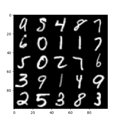
Test Image for Image Detection
Next, we shall train a newly created SVM like in the previous section. However, given that we are now addressing a detection problem, the ground truth labels should not correspond to the digits in the images; instead, they should distinguish between the positive and the negative samples in the training set.
Say, for instance, that we are interested in detecting the two occurrences of the 0 digit in the test image. Hence, the images featuring a 0 in the training portion of the dataset are taken to represent the positive samples and distinguished by a class label of 1. All other images belonging to the remaining digits are taken to represent the negative samples and consequently distinguished by a class label of 0.
Once we have the ground truth labels generated, we may proceed to create and train an SVM on the training dataset:
|
1 2 3 4 5 6 7 8 9 10 11 12 13 14 15 16 17 18 19 |
# Generate labels for the positive and negative samples digits_train_labels = ones((digits_train_imgs.shape[0], 1), dtype=int) digits_train_labels[int(digits_train_labels.shape[0] / 10):digits_train_labels.shape[0], :] = 0 # Create a new SVM svm_digits = ml.SVM_create() # Set the SVM kernel to RBF svm_digits.setKernel(ml.SVM_RBF) svm_digits.setType(ml.SVM_C_SVC) svm_digits.setGamma(0.5) svm_digits.setC(12) svm_digits.setTermCriteria((TERM_CRITERIA_MAX_ITER + TERM_CRITERIA_EPS, 100, 1e-6)) # Convert the training images to HOG descriptors digits_train_hog = hog_descriptors(digits_train_imgs) # Train the SVM on the set of training data svm_digits.train(digits_train_hog, ml.ROW_SAMPLE, digits_train_labels) |
The final piece of code that we shall be adding to the code listing above performs the following operations:
- Traverses the test image by a pre-defined stride.
- Crops an image patch of equivalent size to the sub-images that feature the digits (i.e., 20 $\times$ 20 pixels) from the test image at every iteration.
- Extracts the HOG descriptors of every image patch.
- Feeds the HOG descriptors into the trained SVM to obtain a label prediction.
- Stores the image patch coordinates whenever a detection is found.
- Draws the bounding box for each detection on the original test image.
|
1 2 3 4 5 6 7 8 9 10 11 12 13 14 15 16 17 18 19 20 21 22 23 24 25 26 27 28 29 30 31 32 33 34 35 |
# Create an empty list to store the matching patch coordinates positive_patches = [] # Define the stride to shift with stride = 5 # Iterate over the test image for i in range(0, test_img.shape[0] - 20 + stride, stride): for j in range(0, test_img.shape[1] - 20 + stride, stride): # Crop a patch from the test image patch = test_img[i:i + 20, j:j + 20].reshape(1, 400) # Convert the image patch into HOG descriptors patch_hog = hog_descriptors(patch) # Predict the target label of the image patch _, patch_pred = svm_digits.predict(patch_hog.astype(float32)) # If a match is found, store its coordinate values if patch_pred == 1: positive_patches.append((i, j)) # Convert the list to an array positive_patches = array(positive_patches) # Iterate over the match coordinates and draw their bounding box for i in range(positive_patches.shape[0]): rectangle(test_img, (positive_patches[i, 1], positive_patches[i, 0]), (positive_patches[i, 1] + 20, positive_patches[i, 0] + 20), 255, 1) # Display the test image imshow(test_img, cmap='gray') show() |
The complete code listing is as follows:
|
1 2 3 4 5 6 7 8 9 10 11 12 13 14 15 16 17 18 19 20 21 22 23 24 25 26 27 28 29 30 31 32 33 34 35 36 37 38 39 40 41 42 43 44 45 46 47 48 49 50 51 52 53 54 55 56 57 58 59 60 61 62 63 64 65 66 67 68 69 70 71 72 73 74 75 76 77 78 79 80 81 82 83 84 85 86 87 88 89 90 91 92 93 94 95 96 97 98 99 100 101 102 103 104 105 106 107 108 109 110 |
from cv2 import ml, TERM_CRITERIA_MAX_ITER, TERM_CRITERIA_EPS, rectangle from numpy import float32, zeros, ones, uint8, array from matplotlib.pyplot import imshow, show from digits_dataset import split_images, split_data from feature_extraction import hog_descriptors from random import randint, seed, shuffle # Load the digits image img, sub_imgs = split_images('Images/digits.png', 20) # Obtain training and testing datasets from the digits image digits_train_imgs, _, digits_test_imgs, _ = split_data(20, sub_imgs, 0.8) # Create an empty list to store the random numbers rand_nums = [] # Seed the random number generator for repeatability seed(10) # Choose 25 random digits from the testing dataset for i in range(0, digits_test_imgs.shape[0], int(digits_test_imgs.shape[0] / 25)): # Generate a random integer rand = randint(i, int(digits_test_imgs.shape[0] / 25) + i - 1) # Append it to the list rand_nums.append(rand) # Shuffle the order of the generated random integers shuffle(rand_nums) # Read the image data corresponding to the random integers rand_test_imgs = digits_test_imgs[rand_nums, :] # Initialize an array to hold the test image test_img = zeros((100, 100), dtype=uint8) # Start a sub-image counter img_count = 0 # Iterate over the test image for i in range(0, test_img.shape[0], 20): for j in range(0, test_img.shape[1], 20): # Populate the test image with the chosen digits test_img[i:i + 20, j:j + 20] = rand_test_imgs[img_count].reshape(20, 20) # Increment the sub-image counter img_count += 1 # Display the test image imshow(test_img, cmap='gray') show() # Generate labels for the positive and negative samples digits_train_labels = ones((digits_train_imgs.shape[0], 1), dtype=int) digits_train_labels[int(digits_train_labels.shape[0] / 10):digits_train_labels.shape[0], :] = 0 # Create a new SVM svm_digits = ml.SVM_create() # Set the SVM kernel to RBF svm_digits.setKernel(ml.SVM_RBF) svm_digits.setType(ml.SVM_C_SVC) svm_digits.setGamma(0.5) svm_digits.setC(12) svm_digits.setTermCriteria((TERM_CRITERIA_MAX_ITER + TERM_CRITERIA_EPS, 100, 1e-6)) # Convert the training images to HOG descriptors digits_train_hog = hog_descriptors(digits_train_imgs) # Train the SVM on the set of training data svm_digits.train(digits_train_hog, ml.ROW_SAMPLE, digits_train_labels) # Create an empty list to store the matching patch coordinates positive_patches = [] # Define the stride to shift with stride = 5 # Iterate over the test image for i in range(0, test_img.shape[0] - 20 + stride, stride): for j in range(0, test_img.shape[1] - 20 + stride, stride): # Crop a patch from the test image patch = test_img[i:i + 20, j:j + 20].reshape(1, 400) # Convert the image patch into HOG descriptors patch_hog = hog_descriptors(patch) # Predict the target label of the image patch _, patch_pred = svm_digits.predict(patch_hog.astype(float32)) # If a match is found, store its coordinate values if patch_pred == 1: positive_patches.append((i, j)) # Convert the list to an array positive_patches = array(positive_patches) # Iterate over the match coordinates and draw their bounding box for i in range(positive_patches.shape[0]): rectangle(test_img, (positive_patches[i, 1], positive_patches[i, 0]), (positive_patches[i, 1] + 20, positive_patches[i, 0] + 20), 255, 1) # Display the test image imshow(test_img, cmap='gray') show() |
The resulting image shows that we have successfully detected the two occurrences of the 0 digit in the test image:
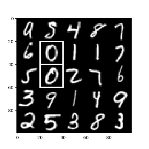
Detecting the Two Occurrences of the 0 Digit
We have considered a simple example, but the same ideas can be easily adapted to address more challenging real-life problems. If you plan to adapt the code above to more challenging problems:
- Remember that the object of interest may appear in various sizes inside the image, so you might need to carry out a multi-scale detection task.
- Do not run into the class imbalance problem when generating positive and negative samples to train your SVM. The examples we have considered in this tutorial were images of very little variation (we were limited to just 10 digits, featuring no variation in scale, lighting, background, etc.), and any dataset imbalance seems to have had very little effect on the detection result. However, real-life challenges do not tend to be this simple, and an imbalanced distribution between classes can lead to poor performance.
Further Reading
This section provides more resources on the topic if you want to go deeper.
Books
- Machine Learning for OpenCV, 2017.
- Mastering OpenCV 4 with Python, 2019.
Websites
- Introduction to Support Vector Machines, https://docs.opencv.org/4.x/d1/d73/tutorial_introduction_to_svm.html
Summary
In this tutorial, you learned how to apply OpenCV’s Support Vector Machine algorithm to solve image classification and detection problems.
Specifically, you learned:
- Several of the most important characteristics of Support Vector Machines.
- How to apply Support Vector Machines to the problems of image classification and detection.
Do you have any questions?
Ask your questions in the comments below, and I will do my best to answer.
Get Started on Machine Learning in OpenCV!
Learn how to use machine learning techniques in image processing projects
...using OpenCV in advanced ways and work beyond pixels
Discover how in my new Ebook:
Machine Learing in OpenCV
It provides self-study tutorials with all working code in Python to turn you from a novice to expert. It equips you with
logistic regression, random forest, SVM, k-means clustering, neural networks,
and much more...all using the machine learning module in OpenCV


")
")
")

No comments yet.