The Support Vector Machine algorithm is one of the most popular supervised machine learning techniques, and it is implemented in the OpenCV library.
This tutorial will introduce the necessary skills to start using Support Vector Machines in OpenCV, using a custom dataset we will generate. In a subsequent tutorial, we will then apply these skills for the specific applications of image classification and detection.
In this tutorial, you will learn how to apply OpenCV’s Support Vector Machine algorithm on a custom two-dimensional dataset.
After completing this tutorial, you will know:
- Several of the most important characteristics of Support Vector Machines.
- How to use the Support Vector Machine algorithm on a custom dataset in OpenCV.
Kick-start your project with my book Machine Learning in OpenCV. It provides self-study tutorials with working code.
Let’s get started.

Support Vector Machines in OpenCV
Photo by Lance Asper, some rights reserved.
Tutorial Overview
This tutorial is divided into two parts; they are:
- Reminder of How Support Vector Machines Work
- Discovering the SVM Algorithm in OpenCV
Reminder of How Support Vector Machines Work
The Support Vector Machine (SVM) algorithm has already been explained well in this tutorial by Jason Brownlee, but let’s first start with brushing up some of the most important points from his tutorial:
- For simplicity, let’s say that we have two separate classes, 0 and 1. A hyperplane can separate the data points within these two classes, the decision boundary that splits the input space to separate the data points by their class. The dimension of this hyperplane depends on the dimensionality of the input data points.
- If given a newly observed data point, we may find the class to which it belongs by calculating which side of the hyperplane it falls.
- A margin is the distance between the decision boundary and the closest data points. It is found by considering only the closest data points belonging to the different classes. It is calculated as the perpendicular distance of these nearest data points to the decision boundary.
- The largest margin to the closest data points characterizes the optimal decision boundary. These nearest data points are known as the support vectors.
- If the classes are not perfectly separable from one another because they may be distributed so that some of their data points intermingle in space, the constraint of maximizing the margin needs to be relaxed. The margin constraint can be relaxed by introducing a tunable parameter known as C.
- The value of the C parameter controls how much the margin constraint can be violated, with a value of 0 meaning that no violation is permitted at all. The aim of increasing the value of C is to reach a better compromise between maximizing the margin and reducing the number of misclassifications.
- Furthermore, the SVM uses a kernel to compute a similarity (or distance) measure between the input data points. In the simplest case, the kernel implements a dot product operation when the input data is linearly separable and can be separated by a linear hyperplane.
- If the data points are not linearly separable straight away, the kernel trick comes to the rescue, where the operation performed by the kernel seeks to transform the data to a higher-dimensional space in which it becomes linearly separable. This is analogous to the SVM finding a non-linear decision boundary in the original input space.
Discovering the SVM algorithm in OpenCV
Let’s first consider applying the SVM to a simple linearly separable dataset that enables us to visualize several of the abovementioned concepts before moving on to more complex tasks.
For this purpose, we shall be generating a dataset consisting of 100 data points (specified by n_samples), which are equally divided into 2 Gaussian clusters (specified by centers) having a standard deviation set to 1.5 (specified by cluster_std). To be able to replicate the results, let’s also define a value for random_state, which we’re going to set to 15:
|
1 2 3 4 5 6 |
# Generate a dataset of 2D data points and their ground truth labels x, y_true = make_blobs(n_samples=100, centers=2, cluster_std=1.5, random_state=15) # Plot the dataset scatter(x[:, 0], x[:, 1], c=y_true) show() |
The code above should generate the following plot of data points. You may note that we are setting the color values to the ground truth labels to be able to distinguish between data points belonging to the two different classes:

Linearly Separable Data Points Belonging to Two Different Classes
The next step is to split the dataset into training and testing sets, where the former will be used to train the SVM and the latter to test it:
|
1 2 3 4 5 6 7 8 9 10 |
# Split the data into training and testing sets x_train, x_test, y_train, y_test = ms.train_test_split(x, y_true, test_size=0.2, random_state=10) # Plot the training and testing datasets fig, (ax1, ax2) = subplots(1, 2) ax1.scatter(x_train[:, 0], x_train[:, 1], c=y_train) ax1.set_title('Training data') ax2.scatter(x_test[:, 0], x_test[:, 1], c=y_test) ax2.set_title('Testing data') show() |
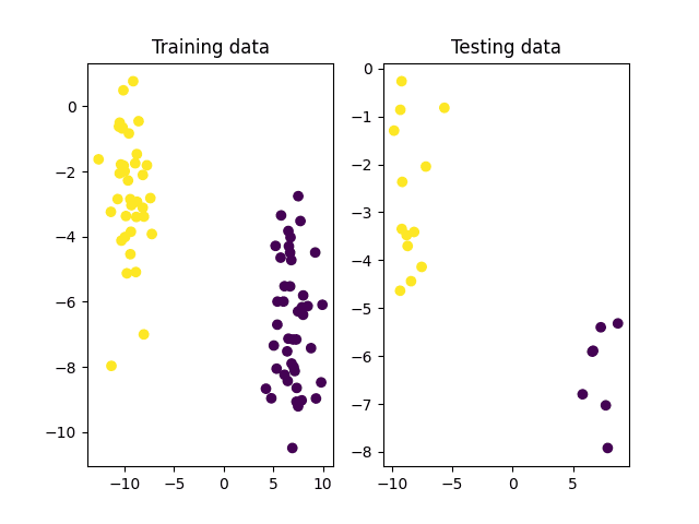
Splitting the Data Points in Training and Testing Sets
We may see from the image of the training data above that the two classes are clearly distinguishable and should be easily separated by a linear hyperplane. Hence, let’s proceed to create and train an SVM in OpenCV that makes use of a linear kernel to find the optimal decision boundary between these two classes:
|
1 2 3 4 5 6 7 8 |
# Create a new SVM svm = ml.SVM_create() # Set the SVM kernel to linear svm.setKernel(ml.SVM_LINEAR) # Train the SVM on the set of training data svm.train(x_train.astype(float32), ml.ROW_SAMPLE, y_train) |
Here, note that the SVM’s train method in OpenCV requires the input data to be of the 32-bit float type.
We may proceed to use the trained SVM to predict labels for the testing data and subsequently calculate the classifier’s accuracy by comparing the predictions with their corresponding ground truth:
|
1 2 3 4 5 6 |
# Predict the target labels of the testing data _, y_pred = svm.predict(x_test.astype(float32)) # Compute and print the achieved accuracy accuracy = (sum(y_pred[:, 0].astype(int) == y_test) / y_test.size) * 100 print('Accuracy:', accuracy, ‘%') |
|
1 |
Accuracy: 100.0 % |
As expected, all of the testing data points have been correctly classified. Let’s also visualize the decision boundary computed by the SVM algorithm during training to understand better how it arrived at this classification result.
In the meantime, the code listing so far is as follows:
|
1 2 3 4 5 6 7 8 9 10 11 12 13 14 15 16 17 18 19 20 21 22 23 24 25 26 27 28 29 30 31 32 33 34 35 36 37 38 39 |
from sklearn.datasets import make_blobs from sklearn import model_selection as ms from numpy import float32 from matplotlib.pyplot import scatter, show, subplots # Generate a dataset of 2D data points and their ground truth labels x, y_true = make_blobs(n_samples=100, centers=2, cluster_std=1.5, random_state=15) # Plot the dataset scatter(x[:, 0], x[:, 1], c=y_true) show() # Split the data into training and testing sets x_train, x_test, y_train, y_test = ms.train_test_split(x, y_true, test_size=0.2, random_state=10) # Plot the training and testing datasets fig, (ax1, ax2) = subplots(1, 2) ax1.scatter(x_train[:, 0], x_train[:, 1], c=y_train) ax1.set_title('Training data') ax2.scatter(x_test[:, 0], x_test[:, 1], c=y_test) ax2.set_title('Testing data') show() # Create a new SVM svm = ml.SVM_create() # Set the SVM kernel to linear svm.setKernel(ml.SVM_LINEAR) # Train the SVM on the set of training data svm.train(x_train.astype(float32), ml.ROW_SAMPLE, y_train) # Predict the target labels of the testing data _, y_pred = svm.predict(x_test.astype(float32)) # Compute and print the achieved accuracy accuracy = (sum(y_pred[:, 0].astype(int) == y_test) / y_test.size) * 100 print('Accuracy:', accuracy, '%') |
To visualize the decision boundary, we will be creating many two-dimensional points structured into a rectangular grid, which span the space occupied by the data points used for testing:
|
1 2 |
x_bound, y_bound = meshgrid(arange(x_test[:, 0].min() - 1, x_test[:, 0].max() + 1, 0.05), arange(x_test[:, 1].min() - 1, x_test[:, 1].max() + 1, 0.05)) |
Next, we shall organize the x- and y-coordinates of the data points that make up the rectangular grid into a two-column array and pass them on to the predict method to generate a class label for each one of them:
|
1 2 |
bound_points = column_stack((x_bound.reshape(-1, 1), y_bound.reshape(-1, 1))).astype(float32) _, bound_pred = svm.predict(bound_points) |
We may finally visualize them by a contour plot overlayed with the data points used for testing to confirm that, indeed, the decision boundary computed by the SVM algorithm is linear:
|
1 2 3 |
contourf(x_bound, y_bound, bound_pred.reshape(x_bound.shape), cmap=cm.coolwarm) scatter(x_test[:, 0], x_test[:, 1], c=y_test) show() |
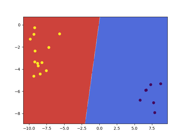
Linear Decision Boundary Computed by the SVM
We may also confirm from the figure above that, as mentioned in the first section, the testing data points have been assigned a class label depending on the side of the decision boundary they were found on.
Furthermore, we may highlight the training data points that have been identified as the support vectors and which have played an instrumental role in determining the decision boundary:
|
1 2 3 4 5 |
support_vect = svm.getUncompressedSupportVectors() scatter(x[:, 0], x[:, 1], c=y_true) scatter(support_vect[:, 0], support_vect[:, 1], c='red') show() |
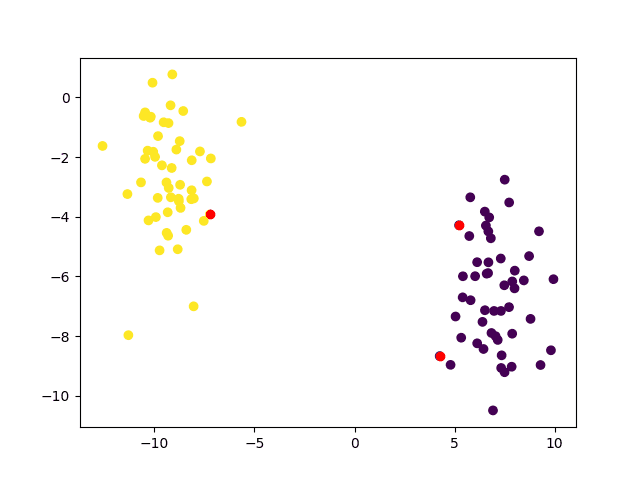
Support Vectors Highlighted in Red
The complete code listing to generate the decision boundary and visualize the support vectors is as follows:
|
1 2 3 4 5 6 7 8 9 10 11 12 13 14 15 16 17 18 19 20 |
from numpy import float32, meshgrid, arange, column_stack from matplotlib.pyplot import scatter, show, contourf, cm x_bound, y_bound = meshgrid(arange(x_test[:, 0].min() - 1, x_test[:, 0].max() + 1, 0.05), arange(x_test[:, 1].min() - 1, x_test[:, 1].max() + 1, 0.05)) bound_points = column_stack((x_bound.reshape(-1, 1), y_bound.reshape(-1, 1))).astype(float32) _, bound_pred = svm.predict(bound_points) # Plot the testing set contourf(x_bound, y_bound, bound_pred.reshape(x_bound.shape), cmap=cm.coolwarm) scatter(x_test[:, 0], x_test[:, 1], c=y_test) show() support_vect = svm.getUncompressedSupportVectors() scatter(x[:, 0], x[:, 1], c=y_true) scatter(support_vect[:, 0], support_vect[:, 1], c='red') show() |
So far, we have considered the simplest case of having two well-distinguishable classes. But how do we distinguish between classes that are less clearly separable because they consist of data points that intermingle in space, such as the following:
|
1 2 |
# Generate a dataset of 2D data points and their ground truth labels x, y_true = make_blobs(n_samples=100, centers=2, cluster_std=8, random_state=15) |
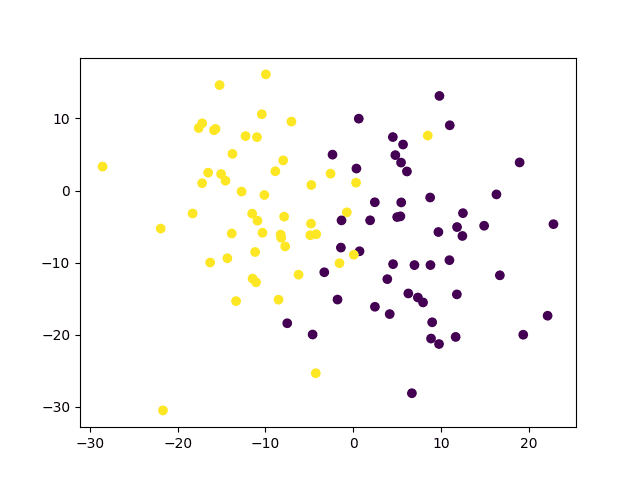
Non-Linearly Separable Data Points Belonging to Two Different Classes
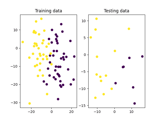
Splitting the Non-Linearly Separable Data in Training and Testing Sets
In this case, we might wish to explore different options depending on how much the two classes overlap one another, such as (1) relaxing the margin constraint for the linear kernel by increasing the value of the C parameter to allow for a better compromise between maximizing the margin and reducing misclassifications, or (2) using a different kernel function that can produce a non-linear decision boundary, such as the Radial Basis Function (RBF).
In doing so, we need to set the values of a few properties of the SVM and the kernel function in use:
- SVM_C_SVC: Known as C-Support Vector Classification, this SVM type allows an n-class classification (n $\geq$ 2) of classes with imperfect separation (i.e. not linearly separable). Set using the
setTypemethod.
- C: Penalty multiplier for outliers when dealing with non-linearly separable classes. Set using the
setCmethod.
- Gamma: Determines the radius of the RBF kernel function. A smaller gamma value results in a wider radius that can capture the similarity of data points far from each other but may result in overfitting. A larger gamma results in a narrower radius that can only capture the similarity of nearby data points, which may result in underfitting. Set using the
setGammamethod.
Here, the C and gamma values are being set arbitrarily, but you may conduct further testing to investigate how different values affect the resulting prediction accuracy. Both of the aforementioned options give us a prediction accuracy of 85% using the following code, but achieve this accuracy through different decision boundaries:
- Using a linear kernel with a relaxed margin constraint:
|
1 2 3 |
svm.setKernel(ml.SVM_LINEAR) svm.setType(ml.SVM_C_SVC) svm.setC(10) |
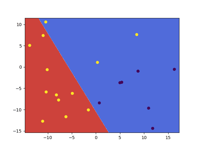
Decision Boundary Computed Using a Linear Kernel with Relaxed Margin Constraints
- Using an RBF kernel function:
|
1 2 3 4 |
svm.setKernel(ml.SVM_RBF) svm.setType(ml.SVM_C_SVC) svm.setC(10) svm.setGamma(0.1) |
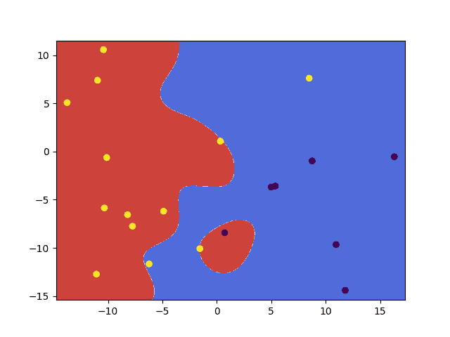
Decision Boundary Computed Using an RBF Kernel
The choice of values for the SVM parameters typically depends on the task and the data at hand and requires further testing to be tuned accordingly.
Further Reading
This section provides more resources on the topic if you want to go deeper.
Books
- Machine Learning for OpenCV, 2017.
- Mastering OpenCV 4 with Python, 2019.
Websites
- Introduction to Support Vector Machines, https://docs.opencv.org/4.x/d1/d73/tutorial_introduction_to_svm.html
Summary
In this tutorial, you learned how to apply OpenCV’s Support Vector Machine algorithm on a custom two-dimensional dataset.
Specifically, you learned:
- Several of the most important characteristics of the Support Vector Machine algorithm.
- How to use the Support Vector Machine algorithm on a custom dataset in OpenCV.
Do you have any questions?
Ask your questions in the comments below, and I will do my best to answer.
Get Started on Machine Learning in OpenCV!
Learn how to use machine learning techniques in image processing projects
...using OpenCV in advanced ways and work beyond pixels
Discover how in my new Ebook:
Machine Learing in OpenCV
It provides self-study tutorials with all working code in Python to turn you from a novice to expert. It equips you with
logistic regression, random forest, SVM, k-means clustering, neural networks,
and much more...all using the machine learning module in OpenCV

")
")
")


No comments yet.