In a previous tutorial, we explored logistic regression as a simple but popular machine learning algorithm for binary classification implemented in the OpenCV library.
So far, we have seen how logistic regression may be applied to a custom two-class dataset we have generated ourselves.
In this tutorial, you will learn how the standard logistic regression algorithm, inherently designed for binary classification, can be modified to cater to multi-class classification problems by applying it to an image classification task.
After completing this tutorial, you will know:
- Several of the most important characteristics of the logistic regression algorithm.
- How the logistic regression algorithm can be modified for multi-class classification problems.
- How to apply logistic regression to the problem of image classification.
Kick-start your project with my book Machine Learning in OpenCV. It provides self-study tutorials with working code.
Let’s get started.

Logistic Regression for Image Classification Using OpenCV
Photo by David Marcu, some rights reserved.
Tutorial Overview
This tutorial is divided into three parts; they are:
- Recap of What Logistic Regression Is
- Modifying Logistic Regression for Multi-Class Classification Problems
- Applying Logistic Regression to a Multi-Class Classification Problem
Recap of What Logistic Regression Is
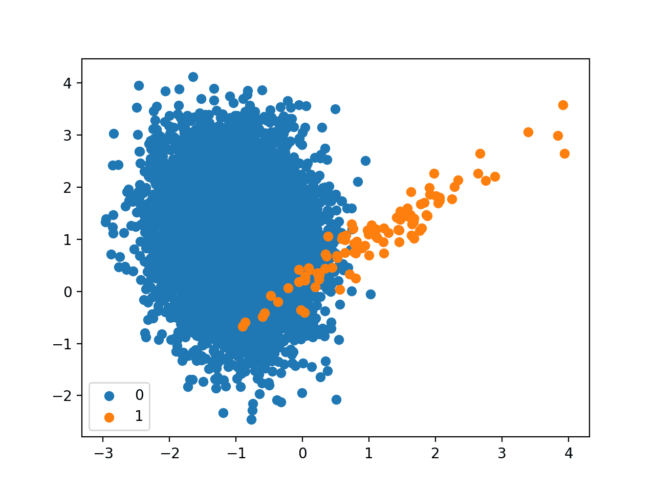
In a previous tutorial, we started exploring OpenCV’s implementation of the logistic regression algorithm. So far, we have applied it to a custom two-class dataset that we have generated, consisting of two-dimensional points gathered into two clusters.
Following Jason Brownlee’s tutorials on logistic regression, we have also recapped the important points about logistic regression. We have seen that logistic regression is closely related to linear regression because they both involve a linear combination of features in generating a real-valued output. However, logistic regression extends this process by applying the logistic (or sigmoid) function. Hence its name. It is to map the real-valued output into a probability value within a range [0, 1]. This probability value is then classified as belonging to the default class if it exceeds a threshold of 0.5; otherwise, it is classified as belonging to the non-default class. This makes logistic regression inherently a method for binary classification.
The logistic regression model is represented by as many coefficients as features in the input data, plus an extra bias value. These coefficients and bias values are learned during training using gradient descent or maximum likelihood estimation (MLE) techniques.
Modifying Logistic Regression for Multi-Class Classification Problems
As mentioned in the previous section, the standard logistic regression method caters solely to two-class problems by how the logistic function and the ensuing thresholding process map the real-valued output of the linear combination of features into either class 0 or class 1.
Hence, catering for multi-class classification problems (or problems that involve more than two classes) with logistic regression requires modification of the standard algorithm.
One technique to achieve this involves splitting the multi-class classification problem into multiple binary (or two-class) classification subproblems. The standard logistic regression method can then be applied to each subproblem. This is how OpenCV implements multi-class logistic regression:
… Logistic Regression supports both binary and multi-class classifications (for multi-class it creates a multiple 2-class classifiers).
A technique of this type is known as the one-vs-one approach, which involves training a separate binary classifier for each unique pair of classes in the dataset. During prediction, each of these binary classifiers votes for one of the two classes on which it was trained, and the class that receives the most votes across all classifiers is taken to be the predicted class.
There are other techniques to achieve multi-class classification with logistic regression, such as through the one-vs-rest approach. You may find further information in these tutorials [1, 2].
Applying Logistic Regression to a Multi-Class Classification Problem
For this purpose, we shall be using the digits dataset in OpenCV, although the code we will develop may also be applied to other multi-class datasets.
Our first step is to load the OpenCV digits image, divide it into its many sub-images that feature handwritten digits from 0 to 9, and create their corresponding ground truth labels that will enable us to quantify the accuracy of the trained logistic regression model later. For this particular example, we will allocate 80% of the dataset images to the training set and the remaining 20% of the images to the testing set:
|
1 2 3 4 5 |
# Load the digits image img, sub_imgs = split_images('Images/digits.png', 20) # Obtain training and testing datasets from the digits image digits_train_imgs, digits_train_labels, digits_test_imgs, digits_test_labels = split_data(20, sub_imgs, 0.8) |
Next, we shall follow a process similar to what we did in the previous tutorial, where we trained and tested the logistic regression algorithm on a two-class dataset, changing a few parameters to adapt it to a larger multi-class dataset.
The first step is, again, to create the logistic regression model itself:
|
1 2 |
# Create an empty logistic regression model lr_digits = ml.LogisticRegression_create() |
We may, again, confirm that OpenCV implements Batch Gradient Descent as its default training method (represented by a value of 0) and then proceed to change this to a Mini-Batch Gradient Descent method, specifying the mini-batch size:
|
1 2 3 4 5 6 |
# Check the default training method print('Training Method:', lr_digits.getTrainMethod()) # Set the training method to Mini-Batch Gradient Descent and the size of the mini-batch lr_digits.setTrainMethod(ml.LogisticRegression_MINI_BATCH) lr_digits.setMiniBatchSize(400) |
Different mini-batch sizes will certainly affect the model’s training and prediction accuracy.
Our choice for the mini-batch size in this example was based on a heuristic approach for practicality, whereby a few mini-batch sizes were experimented with, and a value that resulted in a sufficiently high prediction accuracy (as we will see later) was identified. However, you should follow a more systematic approach, which can provide you with a more informed decision about the mini-batch size that offers a better compromise between computational cost and prediction accuracy for the task at hand.
Next, we shall define the number of iterations that we want to run the chosen training algorithm for before it terminates:
|
1 2 |
# Set the number of iterations lr.setIterations(10) |
We’re now set to train the logistic regression model on the training data:
|
1 2 |
# Train the logistic regressor on the set of training data lr_digits.train(digits_train_imgs.astype(float32), ml.ROW_SAMPLE, digits_train_labels.astype(float32)) |
In our previous tutorial, we printed out the learned coefficients to discover how the model, which best separated the two-class samples we worked with, was defined.
We shall not be printing out the learned coefficients this time round, mainly because there are too many of them, given that we are now working with input data of higher dimensionality.
What we shall alternatively do is print out the number of learned coefficients (rather than the coefficients themselves) as well as the number of input features to be able to compare the two:
|
1 2 3 |
# Print the number of learned coefficients, and the number of input features print('Number of coefficients:', len(lr_digits.get_learnt_thetas()[0])) print('Number of input features:', len(digits_train_imgs[0, :])) |
|
1 2 |
Number of coefficients: 401 Number of input features: 400 |
Indeed, we find that we have as many coefficient values as input features, plus an additional bias value, as we had expected (we are working with $20\times 20$ pixel images, and we are using the pixel values themselves as the input features, hence 400 features per image).
We can test how well this model predicts the target class labels by trying it out on the testing part of the dataset:
|
1 2 3 4 5 6 |
# Predict the target labels of the testing data _, y_pred = lr_digits.predict(digits_test_imgs.astype(float32)) # Compute and print the achieved accuracy accuracy = (sum(y_pred[:, 0] == digits_test_labels[:, 0]) / digits_test_labels.size) * 100 print('Accuracy:', accuracy, '%') |
|
1 |
Accuracy: 88.8 % |
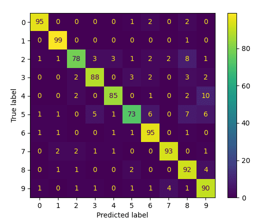
As a final step, let’s go ahead to generate and plot a confusion matrix to gain a deeper insight into which digits have been mistaken for one another:
|
1 2 3 4 5 |
# Generate and plot confusion matrix cm = confusion_matrix(digits_test_labels, y_pred) disp = ConfusionMatrixDisplay(confusion_matrix=cm) disp.plot() show() |
In this manner, we can see that the classes with the lowest performance are 5 and 2, which are mistaken mostly for 8.
The entire code listing is as follows:
|
1 2 3 4 5 6 7 8 9 10 11 12 13 14 15 16 17 18 19 20 21 22 23 24 25 26 27 28 29 30 31 32 33 34 35 36 37 38 39 40 41 42 43 44 45 46 |
from cv2 import ml from sklearn.datasets import make_blobs from sklearn import model_selection as ms from sklearn.metrics import confusion_matrix, ConfusionMatrixDisplay from numpy import float32 from matplotlib.pyplot import show from digits_dataset import split_images, split_data # Load the digits image img, sub_imgs = split_images('Images/digits.png', 20) # Obtain training and testing datasets from the digits image digits_train_imgs, digits_train_labels, digits_test_imgs, digits_test_labels = split_data(20, sub_imgs, 0.8) # Create an empty logistic regression model lr_digits = ml.LogisticRegression_create() # Check the default training method print('Training Method:', lr_digits.getTrainMethod()) # Set the training method to Mini-Batch Gradient Descent and the size of the mini-batch lr_digits.setTrainMethod(ml.LogisticRegression_MINI_BATCH) lr_digits.setMiniBatchSize(400) # Set the number of iterations lr_digits.setIterations(10) # Train the logistic regressor on the set of training data lr_digits.train(digits_train_imgs.astype(float32), ml.ROW_SAMPLE, digits_train_labels.astype(float32)) # Print the number of learned coefficients, and the number of input features print('Number of coefficients:', len(lr_digits.get_learnt_thetas()[0])) print('Number of input features:', len(digits_train_imgs[0, :])) # Predict the target labels of the testing data _, y_pred = lr_digits.predict(digits_test_imgs.astype(float32)) # Compute and print the achieved accuracy accuracy = (sum(y_pred[:, 0] == digits_test_labels[:, 0]) / digits_test_labels.size) * 100 print('Accuracy:', accuracy, '%') # Generate and plot confusion matrix cm = confusion_matrix(digits_test_labels, y_pred) disp = ConfusionMatrixDisplay(confusion_matrix=cm) disp.plot() show() |
In this tutorial, we have applied the logistic regression method, inherently designed for binary classification, to a multi-class classification problem. We have used the pixel values as input features representing each image, obtaining an 88.8% classification accuracy with the chosen parameter values.
How about testing whether training the logistic regression algorithm on HOG descriptors extracted from the images would improve this accuracy?
Want to Get Started With Machine Learning with OpenCV?
Take my free email crash course now (with sample code).
Click to sign-up and also get a free PDF Ebook version of the course.
Further Reading
This section provides more resources on the topic if you want to go deeper.
Books
- Machine Learning for OpenCV, 2017.
- Mastering OpenCV 4 with Python, 2019.
Websites
- Logistic Regression, https://docs.opencv.org/3.4/dc/dd6/ml_intro.html#ml_intro_lr
Summary
In this tutorial, you learned how the standard logistic regression algorithm, inherently designed for binary classification, can be modified to cater to multi-class classification problems by applying it to an image classification task.
Specifically, you learned:
- Several of the most important characteristics of the logistic regression algorithm.
- How the logistic regression algorithm can be modified for multi-class classification problems.
- How to apply logistic regression to the problem of image classification.
Do you have any questions?
Ask your questions in the comments below, and I will do my best to answer.


No comments yet.