A sample of data is a snapshot from a broader population of all possible observations that could be taken of a domain or generated by a process.
Interestingly, many observations fit a common pattern or distribution called the normal distribution, or more formally, the Gaussian distribution. A lot is known about the Gaussian distribution, and as such, there are whole sub-fields of statistics and statistical methods that can be used with Gaussian data.
In this tutorial, you will discover the Gaussian distribution, how to identify it, and how to calculate key summary statistics of data drawn from this distribution.
After completing this tutorial, you will know:
That the Gaussian distribution describes many observations, including many observations seen during applied machine learning.
That the central tendency of a distribution is the most likely observation and can be estimated from a sample of data as the mean or median.
That the variance is the average deviation from the mean in a distribution and can be estimated from a sample of data as the variance and standard deviation.
Kick-start your project with my new book Statistics for Machine Learning, including step-by-step tutorials and the Python source code files for all examples.
Let’s get started.
A Gentle Introduction to Calculating Normal Summary Statistics Photo by John, some rights reserved.
Tutorial Overview
This tutorial is divided into 6 parts; they are:
Gaussian Distribution
Sample vs Population
Test Dataset
Central Tendencies
Variance
Describing a Gaussian
Need help with Statistics for Machine Learning?
Take my free 7-day email crash course now (with sample code).
Click to sign-up and also get a free PDF Ebook version of the course.
Gaussian Distribution
A distribution of data refers to the shape it has when you graph it, such as with a histogram.
The most commonly seen and therefore well-known distribution of continuous values is the bell curve. It is known as the “normal” distribution, because it the distribution that a lot of data falls into. It is also known as the Gaussian distribution, more formally, named for Carl Friedrich Gauss.
As such, you will see references to data being normally distributed or Gaussian, which are interchangeable, both referring to the same thing: that the data looks like the Gaussian distribution.
Some examples of observations that have a Gaussian distribution include:
People’s heights.
IQ scores.
Body temperature.
Let’s look at a normal distribution. Below is some code to generate and plot an idealized Gaussian distribution.
1
2
3
4
5
6
7
8
9
10
11
# generate and plot an idealized gaussian
from numpy import arange
from matplotlib import pyplot
from scipy.stats import norm
# x-axis for the plot
x_axis=arange(-3,3,0.001)
# y-axis as the gaussian
y_axis=norm.pdf(x_axis,0,1)
# plot data
pyplot.plot(x_axis,y_axis)
pyplot.show()
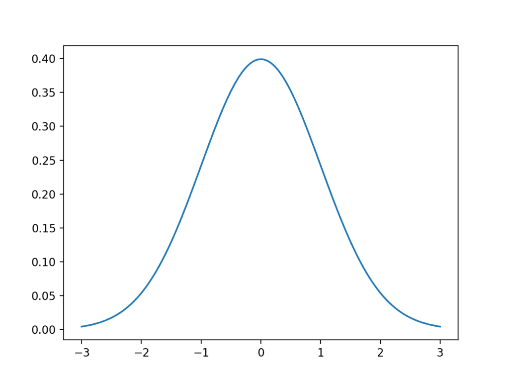
Running the example generates a plot of an idealized Gaussian distribution.
The x-axis are the observations and the y-axis is the frequency of each observation. In this case, observations around 0.0 are the most common and observations around -3.0 and 3.0 are rare or unlikely.
Line Plot of Gaussian Distribution
It is helpful when data is Gaussian or when we assume a Gaussian distribution for calculating statistics. This is because the Gaussian distribution is very well understood. So much so that large parts of the field of statistics are dedicated to methods for this distribution.
Thankfully, many of the data we work with in machine learning often fits a Gaussian distribution, such as the input data we may use to fit a model, to the repeated evaluation of a model on different samples of training data.
Not all data is Gaussian, and it is sometimes important to make this discovery either by reviewing histogram plots of the data or using statistical tests to check. Some examples of observations that do not fit a Gaussian distribution include:
People’s incomes.
Population of cities.
Sales of books.
Sample vs Population
We can think of data being generated by some unknown process.
The data that we collect is called a data sample, whereas all possible data that could be collected is called the population.
Data Sample: A subset of observations from a group.
Data Population: All possible observations from a group.
This is an important distinction because different statistical methods are used on samples vs populations, and in applied machine learning, we are often working with samples of data. If you read or use the word “population” when talking about data in machine learning, it very likely means sample when it comes to statistical methods.
Two examples of data samples that you will encounter in machine learning include:
The train and test datasets.
The performance scores for a model.
When using statistical methods, we often want to make claims about the population using only observations in the sample.
Two clear examples of this include:
The training sample must be representative of the population of observations so that we can fit a useful model.
The test sample must be representative of the population of observations so that we can develop an unbiased evaluation of the model skill.
Because we are working with samples and making claims about a population, it means that there is always some uncertainty, and it is important to understand and report this uncertainty.
Test Dataset
Before we explore some important summary statistics for data with a Gaussian distribution, let’s first generate a sample of data that we can work with.
We can use the randn() NumPy function to generate a sample of random numbers drawn from a Gaussian distribution.
There are two key parameters that define any Gaussian distribution; they are the mean and the standard deviation. We will go more into these parameters later as they are also key statistics to estimate when we have data drawn from an unknown Gaussian distribution.
The randn() function will generate a specified number of random numbers (e.g. 10,000) drawn from a Gaussian distribution with a mean of zero and a standard deviation of 1. We can then scale these numbers to a Gaussian of our choosing by rescaling the numbers.
This can be made consistent by adding the desired mean (e.g. 50) and multiplying the value by the standard deviation (5).
1
data=5*randn(10000)+50
We can then plot the dataset using a histogram and look for the expected shape of the plotted data.
The complete example is listed below.
1
2
3
4
5
6
7
8
9
10
11
# generate a sample of random gaussians
from numpy.random import seed
from numpy.random import randn
from matplotlib import pyplot
# seed the random number generator
seed(1)
# generate univariate observations
data=5*randn(10000)+50
# histogram of generated data
pyplot.hist(data)
pyplot.show()
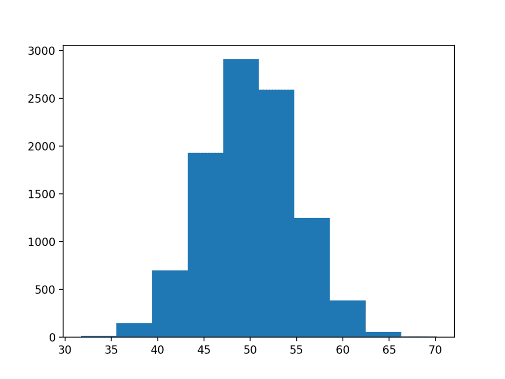
Running the example generates the dataset and plots it as a histogram.
We can almost see the Gaussian shape to the data, but it is blocky. This highlights an important point.
Sometimes, the data will not be a perfect Gaussian, but it will have a Gaussian-like distribution. It is almost Gaussian and maybe it would be more Gaussian if it was plotted in a different way, scaled in some way, or if more data was gathered.
Often, when working with Gaussian-like data, we can treat it as Gaussian and use all of the same statistical tools and get reliable results.
Histogram plot of Gaussian Dataset
In the case of this dataset, we do have enough data and the plot is blocky because the plotting function chooses an arbitrary sized bucket for splitting up the data. We can choose a different, more granular way to split up the data and better expose the underlying Gaussian distribution.
The updated example with the more refined plot is listed below.
1
2
3
4
5
6
7
8
9
10
11
# generate a sample of random gaussians
from numpy.random import seed
from numpy.random import randn
from matplotlib import pyplot
# seed the random number generator
seed(1)
# generate univariate observations
data=5*randn(10000)+50
# histogram of generated data
pyplot.hist(data,bins=100)
pyplot.show()
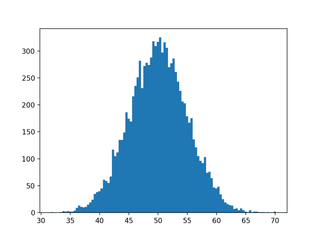
Running the example, we can see that choosing 100 splits of the data does a much better job of creating a plot that clearly shows the Gaussian distribution of the data.
The dataset was generated from a perfect Gaussian, but the numbers were randomly chosen and we only chose 10,000 observations for our sample. You can see, even with this controlled setup, there is obvious noise in the data sample.
This highlights another important point: that we should always expect some noise or limitation in our data sample. The data sample will always contain errors compared to the pure underlying distribution.
Histogram plot of Gaussian Dataset With More Bins
Central Tendency
The central tendency of a distribution refers to the middle or typical value in the distribution. The most common or most likely value.
In the Gaussian distribution, the central tendency is called the mean, or more formally, the arithmetic mean, and is one of the two main parameters that defines any Gaussian distribution.
The mean of a sample is calculated as the sum of the observations divided by the total number of observations in the sample.
1
mean=sum(data)/length(data)
It is also written in a more compact form as:
1
mean = 1 / length(data) * sum(data)
We can calculate the mean of a sample by using the mean() NumPy function on an array.
1
result=mean(data)
The example below demonstrates this on the test dataset developed in the previous section.
1
2
3
4
5
6
7
8
9
10
11
# calculate the mean of a sample
from numpy.random import seed
from numpy.random import randn
from numpy import mean
# seed the random number generator
seed(1)
# generate univariate observations
data=5*randn(10000)+50
# calculate mean
result=mean(data)
print('Mean: %.3f'%result)
Running the example calculates and prints the mean of the sample.
This calculation of the arithmetic mean of the sample is an estimate of the parameter of the underlying Gaussian distribution of the population from which the sample was drawn. As an estimate, it will contain errors.
Because we know the underlying distribution has the true mean of 50, we can see that the estimate from a sample of 10,000 observations is reasonably accurate.
1
Mean: 50.049
The mean is easily influenced by outlier values, that is, rare values far from the mean. These may be legitimately rare observations on the edge of the distribution or errors.
Further, the mean may be misleading. Calculating a mean on another distribution, such as a uniform distribution or power distribution, may not make a lot of sense as although the value can be calculated, it will refer to a seemingly arbitrary expected value rather than the true central tendency of the distribution.
In the case of outliers or a non-Gaussian distribution, an alternate and commonly used central tendency to calculate is the median.
The median is calculated by first sorting all data and then locating the middle value in the sample. This is straightforward if there is an odd number of observations. If there is an even number of observations, the median is calculated as the average of the middle two observations.
We can calculate the median of a sample of an array by calling the median() NumPy function.
1
result=median(data)
The example below demonstrates this on the test dataset.
1
2
3
4
5
6
7
8
9
10
11
# calculate the median of a sample
from numpy.random import seed
from numpy.random import randn
from numpy import median
# seed the random number generator
seed(1)
# generate univariate observations
data=5*randn(10000)+50
# calculate median
result=median(data)
print('Median: %.3f'%result)
Running the example, we can see that median is calculated from the sample and printed.
The result is not too dissimilar from the mean because the sample has a Gaussian distribution. If the data had a different (non-Gaussian) distribution, the median may be very different from the mean and perhaps a better reflection of the central tendency of the underlying population.
1
Median:50.042
Variance
The variance of a distribution refers to how much on average that observations vary or differ from the mean value.
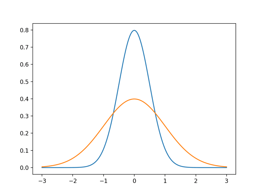
It is useful to think of the variance as a measure of the spread of a distribution. A low variance will have values grouped around the mean (e.g. a narrow bell shape), whereas a high variance will have values spread out from the mean (e.g. a wide bell shape.)
We can demonstrate this with an example, by plotting idealized Gaussians with low and high variance. The complete example is listed below.
1
2
3
4
5
6
7
8
9
10
11
# generate and plot gaussians with different variance
from numpy import arange
from matplotlib import pyplot
from scipy.stats import norm
# x-axis for the plot
x_axis=arange(-3,3,0.001)
# plot low variance
pyplot.plot(x_axis,norm.pdf(x_axis,0,0.5))
# plot high variance
pyplot.plot(x_axis,norm.pdf(x_axis,0,1))
pyplot.show()
Running the example plots two idealized Gaussian distributions: the blue with a low variance grouped around the mean and the orange with a higher variance with more spread.
Line plot of Gaussian distributions with low and high variance
The variance of a data sample drawn from a Gaussian distribution is calculated as the average squared difference of each observation in the sample from the sample mean:
Where variance is often denoted as s^2 clearly showing the squared units of the measure. You may see the equation without the (- 1) from the number of observations, and this is the calculation of the variance for the population, not the sample.
We can calculate the variance of a data sample in NumPy using the var() function.
The example below demonstrates calculating variance on the test problem.
1
2
3
4
5
6
7
8
9
10
11
# calculate the variance of a sample
from numpy.random import seed
from numpy.random import randn
from numpy import var
# seed the random number generator
seed(1)
# generate univariate observations
data=5*randn(10000)+50
# calculate variance
result=var(data)
print('Variance: %.3f'%result)
Running the example calculates and prints the variance.
1
Variance: 24.939
It is hard to interpret the variance because the units are the squared units of the observations. We can return the units to the original units of the observations by taking the square root of the result.
For example, the square root of 24.939 is about 4.9.
Often, when the spread of a Gaussian distribution is summarized, it is described using the square root of the variance. This is called the standard deviation. The standard deviation, along with the mean, are the two key parameters required to specify any Gaussian distribution.
We can see that the value of 4.9 is very close to the value of 5 for the standard deviation specified when the samples were created for the test problem.
We can wrap the variance calculation in a square root to calculate the standard deviation directly.
Where the standard deviation is often written as s or as the Greek lowercase letter sigma.
The standard deviation can be calculated directly in NumPy for an array via the std() function.
The example below demonstrates the calculation of the standard deviation on the test problem.
1
2
3
4
5
6
7
8
9
10
11
# calculate the standard deviation of a sample
from numpy.random import seed
from numpy.random import randn
from numpy import std
# seed the random number generator
seed(1)
# generate univariate observations
data=5*randn(10000)+50
# calculate standard deviation
result=std(data)
print('Standard Deviation: %.3f'%result)
Running the example calculates and prints the standard deviation of the sample. The value matches the square root of the variance and is very close to 5.0, the value specified in the definition of the problem.
1
Standard Deviation: 4.994
Measures of variance can be calculated for non-Gaussian distributions, but generally require the distribution to be identified so that a specialized measure of variance specific to that distribution can be calculated.
Describing a Gaussian
In applied machine learning, you will often need to report the results of an algorithm.
That is, report the estimated skill of the model on out-of-sample data.
This is often done by reporting the mean performance from a k-fold cross-validation, or some other repeated sampling procedure.
When reporting model skill, you are in effect summarizing the distribution of skill scores, and very likely the skill scores will be drawn from a Gaussian distribution.
It is common to only report the mean performance of the model. This would hide two other important details of the distribution of the skill of the model.
As a minimum I would recommend reporting the two parameters of the Gaussian distribution of model scores and the size of the sample. Ideally, it would also be a good idea to confirm that indeed the model skill scores are Gaussian or look Gaussian enough to defend reporting the parameters of the Gaussian distribution.
This is important because the distribution of skill scores can be reconstructed by readers and potentially compared to the skill of models on the same problem in the future.
Extensions
This section lists some ideas for extending the tutorial that you may wish to explore.
Develop your own test problem and calculate the central tendency and variance measures.
Develop a function to calculate a summary report on a given data sample.
Load and summarize the variables for a standard machine learning dataset
If you explore any of these extensions, I’d love to know.
Further Reading
This section provides more resources on the topic if you are looking to go deeper.
In this tutorial, you discovered the Gaussian distribution, how to identify it, and how to calculate key summary statistics of data drawn from this distribution.
Specifically, you learned:
That the Gaussian distribution describes many observations, including many observations seen during applied machine learning.
That the central tendency of a distribution is the most likely observation and can be estimated from a sample of data as the mean or median.
That the variance is the average deviation from the mean in a distribution and can be estimated from a sample of data as the variance and standard deviation.
Do you have any questions?
Ask your questions in the comments below and I will do my best to answer.
Nice introduction to Gaussian distribution in short duration and practiced in few minutes, Thank you , May I know what are its applications in real Data Science (particularly in Applied Machine learning)
Dear Dr Jason,
I am looking at this tutorial and the other two associated tutorials.
I can plot functions using
1
2
pyplot.plot(x,y);#looks like a continuous plot
pyplot.scatter(x,y);#uses symbols for plotting values.
For histograms I can do the following:
1
pyplot.hist(yaxis);#Don't need the xaxis. The no of bins determines how detailed the hist.
I wouldparticularly like to know about the function
c
Such that I can plot:
pyplot.plot(xaxis, yaxis)
pyplot.show()
Going back to:
1
yaxis=norm.pdf(xaxis,0,0.5)
* I understand that norm..pdf generates a pairwise y-value from the normal distribution for a corresponding x-value. Otherwise if the y-values were not ordered, you’ll get a zig-zagged shaped x-y plot.
* What are the parameters 0 and 0.5 mean, I thought they were the mean and stddev, BUT:
Dear Dr Jason,
I agree with you that it should generate a mean of 0 and stdev of 1.
But when I did
1
2
3
4
5
6
7
>>>np.mean(y)
0.16666666633781846;# DEFINITELY NOT ZERO MEAN
>>>np.std(y)
0.25739817324489317# DEFINITELY NOT STD DEV of 1
In sum when I generated the sequence yaxis from the normal distribution with mean 0 and stddev 0.5, I did not get 0 and 0.5 respectively ,. rather 0.166 and 0.257
In other worrds if I generated the function
1
yaxis=norm.pdf(xaxis,0,0.5)
Why didn’t I get something close to 0 or close to 0.5?
Dear Dr Jason,
When I looked at the abovementioned hyperlinked document at scipy.org, I don’t understand the meaning and APPLICATION of ‘loc’ and ‘scale’ ‘
IN SUM: meaning of ‘loc’ and ‘scale’ AND how to generate a pdf or sequence from the normal distribution with a mean of 0 and std dev of 1.
Dear Dr Jason,
The page https://docs.scipy.org/doc/scipy/reference/generated/scipy.stats.norm.html in the first paragraph says loc = mean, and scale = stddev. Don’t know why ‘they’ could not call the parameters mean and stddev. It should be consistent.OK I can understand and apologise for the oversight.
But the following code based on the subheading ‘Variance’ does not correspond to the desired result under the norm.pdf(x, loc, scale) function.
1
2
3
4
5
6
7
8
9
10
11
12
13
14
15
16
17
18
19
20
21
import numpy asnp
from numpy import arange
from matplotlib import pyplot
from scipy.stats import norm
#
#
#generate the x value
x_axis=arange(-3,3,0.001)
#generate the y value, based on line 10
#generate y value with mean =0, stddev = 1
y_axis=norm.pdf(x_axis,0,1)
#what the mean & stddev of the yaxis
np.mean(y_axis)
0.16621670028682048;#WHY NOT ZERO ACCORDING TO PDF?
np.std(y_axis)
0.13923637660149782;#WHY NOT 1 ACCORDING TO PDFR?
.
Again, if the norm.pdf funtion with loc and scale being respectively 0 and 1, why am I getting the respective mean and stddev of 0.1622 and 0.1392. I’m supposed to get 0 and 1 for my x_axis of length 6000.
I though generating a sequence of 6000 numbers should give me something close to a normal distribution with mean of 0 and stddev of 1. I seem to be missing something.
Dear Dr Jason,
I thank you for averting me to the article on the pdf at https://en.wikipedia.org/wiki/Probability_density_function . I suddenly recalled an intro stats course at university using the z-table. You can work out the probability of an event between two values.
Having had a look at the pdf on the right hand of the wiki page, all this info about the area under the curve between +-1 std dev (x axis) is 68.27%, within +- 2 std dev (x axis) is 95%, and within +- 3 std dev, is 99%.
Understood this perfectly.
So going back to the example, I wanted to calculate the probability of the function between -1 and 1. I expected to have 0.6827. Instead I got 682.7.
1
2
3
4
5
6
7
8
9
10
11
12
13
14
15
16
17
18
19
20
21
22
23
24
import numpy asnp
from numpy import arange
from matplotlib import pyplot
from scipy.stats import norm
#
#
#generate the x value
x_axis=arange(-3,3,0.001)
#generate the y value, based on line 10
#generate y value with mean =0, stddev = 1
y_axis=norm.pdf(x_axis,0,1)
#Select those values of x_axis between -1 and 1 and thus itscorresponding #values of the pdf
selected_values=y_axis[(x_axis>=-1)&(x_axis<=1)]
#calculate the probability as the sum of the selected values,
# Reference wiki article subheading "Absolutely continuous univariate
# distributions
print(np.sum(selected_values))
682.6894518086525
In sum: I understood that you meant pdf. The horizontal axis = x_axis represents the number of std deviations. The vertical axis is the probability for a given value of x.
BUT why do I get the pdf between -1 and 1 std dev to be 682.68945 and not 0.68268945
Superb Jason!
like always; the best part I took home is this:
” …reporting the two parameters of the Gaussian distribution of model scores *and the size of the sample*”


Solid overview. I typically prefer R & the tidyverse for plotting and analysis, but the statistical functions in base R are sort of clumsy.
… Numpy feels more intuitive.
Thanks.
Hi Jason
Kindly pass me your email id so that we can work together, I.m wokeijf in smart surveillance system
You can use the contact me page.
Please see this regarding new projects:
https://machinelearningmastery.com/faq/single-faq/can-you-help-me-with-my-project
Nice introduction to Gaussian distribution in short duration and practiced in few minutes, Thank you , May I know what are its applications in real Data Science (particularly in Applied Machine learning)
It can help you to understand your data prior to pre-processing and modeling.
Hi Jason,
Do you have any book for this tuto (Statistics)?
Yes, I am finalizing one at the moment.
Dear Dr Jason,
I am looking at this tutorial and the other two associated tutorials.
I can plot functions using
For histograms I can do the following:
I wouldparticularly like to know about the function
c
Such that I can plot:
pyplot.plot(xaxis, yaxis)
pyplot.show()
Going back to:
* I understand that norm..pdf generates a pairwise y-value from the normal distribution for a corresponding x-value. Otherwise if the y-values were not ordered, you’ll get a zig-zagged shaped x-y plot.
* What are the parameters 0 and 0.5 mean, I thought they were the mean and stddev, BUT:
I could not find a suitable example to explain the parameters, even https://docs.scipy.org/doc/scipy/reference/generated/scipy.stats.norm.html was vague.
Thank you,
Anthony of exciting Belfield
We are generating a sample of gaussian numbers with a mean of 0 and a stdev of 1. The numbers are ordered by the x-axis.
It is a function transform x as input y as output. The line plot of y shows the bell shape.
Dear Dr Jason,
I agree with you that it should generate a mean of 0 and stdev of 1.
But when I did
In sum when I generated the sequence yaxis from the normal distribution with mean 0 and stddev 0.5, I did not get 0 and 0.5 respectively ,. rather 0.166 and 0.257
In other worrds if I generated the function
Why didn’t I get something close to 0 or close to 0.5?
Thank you
Anthony of Belfield
My mistake, the parameters for pdf() are “loc” and “scale”:
https://docs.scipy.org/doc/scipy/reference/generated/scipy.stats.norm.html
Dear Dr Jason,
When I looked at the abovementioned hyperlinked document at scipy.org, I don’t understand the meaning and APPLICATION of ‘loc’ and ‘scale’ ‘
IN SUM: meaning of ‘loc’ and ‘scale’ AND how to generate a pdf or sequence from the normal distribution with a mean of 0 and std dev of 1.
Thank you,
Anthony from NSW
Dear Dr Jason,
The page https://docs.scipy.org/doc/scipy/reference/generated/scipy.stats.norm.html in the first paragraph says loc = mean, and scale = stddev. Don’t know why ‘they’ could not call the parameters mean and stddev. It should be consistent.OK I can understand and apologise for the oversight.
But the following code based on the subheading ‘Variance’ does not correspond to the desired result under the norm.pdf(x, loc, scale) function.
.
Again, if the norm.pdf funtion with loc and scale being respectively 0 and 1, why am I getting the respective mean and stddev of 0.1622 and 0.1392. I’m supposed to get 0 and 1 for my x_axis of length 6000.
I though generating a sequence of 6000 numbers should give me something close to a normal distribution with mean of 0 and stddev of 1. I seem to be missing something.
What is it?
Thank you,
Anthony of NSW
The function is not generating Gaussian random numbers, it is generating the probability of provided input values on the standard normal.
The distribution of the probabilities will not have a mean of 0 and a stdev of 1.
Does that help?
Here’s more on what a PDF is:
https://en.wikipedia.org/wiki/Probability_density_function
Dear Dr Jason,
I thank you for averting me to the article on the pdf at https://en.wikipedia.org/wiki/Probability_density_function . I suddenly recalled an intro stats course at university using the z-table. You can work out the probability of an event between two values.
Having had a look at the pdf on the right hand of the wiki page, all this info about the area under the curve between +-1 std dev (x axis) is 68.27%, within +- 2 std dev (x axis) is 95%, and within +- 3 std dev, is 99%.
Understood this perfectly.
So going back to the example, I wanted to calculate the probability of the function between -1 and 1. I expected to have 0.6827. Instead I got 682.7.
In sum: I understood that you meant pdf. The horizontal axis = x_axis represents the number of std deviations. The vertical axis is the probability for a given value of x.
BUT why do I get the pdf between -1 and 1 std dev to be 682.68945 and not 0.68268945
Thank you,
Anthony of Belfield
Dear DrJason,
I have posted the same question at this site https://oneau.wordpress.com/2011/02/28/simple-statistics-with-scipy/#comment-2276 and thought I like to share the answer. .
Prasanth gave the answer. In essence you the distance between x is 0.001. So you multiply each corresponding f(x) by 0.001 and then sum the f(x)
So here is the correct implementation:
I knew it was something that simple that I would share it with others,
Regards and thanks
Anthony of exciting Sydney
Superb Jason!
like always; the best part I took home is this:
” …reporting the two parameters of the Gaussian distribution of model scores *and the size of the sample*”
Thanks, I’m glad it helped.
If I’m reading the numpy documentation correctly, it outputs the population std/var by default.
You’ve presented the sample standard deviation / variance formulas that divide by ‘N-1’.
Was this on purpose?
No, thanks for the note.