The XGBoost algorithm is effective for a wide range of regression and classification predictive modeling problems.
It is an efficient implementation of the stochastic gradient boosting algorithm and offers a range of hyperparameters that give fine-grained control over the model training procedure. Although the algorithm performs well in general, even on imbalanced classification datasets, it offers a way to tune the training algorithm to pay more attention to misclassification of the minority class for datasets with a skewed class distribution.
This modified version of XGBoost is referred to as Class Weighted XGBoost or Cost-Sensitive XGBoost and can offer better performance on binary classification problems with a severe class imbalance.
In this tutorial, you will discover weighted XGBoost for imbalanced classification.
After completing this tutorial, you will know:
How gradient boosting works from a high level and how to develop an XGBoost model for classification.
How the XGBoost training algorithm can be modified to weight error gradients proportional to positive class importance during training.
How to configure the positive class weight for the XGBoost training algorithm and how to grid search different configurations.
Kick-start your project with my new book Imbalanced Classification with Python, including step-by-step tutorials and the Python source code files for all examples.
Let’s get started.
How to Configure XGBoost for Imbalanced Classification Photo by flowcomm, some rights reserved.
Tutorial Overview
This tutorial is divided into four parts; they are:
Imbalanced Classification Dataset
XGBoost Model for Classification
Weighted XGBoost for Class Imbalance
Tune the Class Weighting Hyperparameter
Imbalanced Classification Dataset
Before we dive into XGBoost for imbalanced classification, let’s first define an imbalanced classification dataset.
We can use the make_classification() scikit-learn function to define a synthetic imbalanced two-class classification dataset. We will generate 10,000 examples with an approximate 1:100 minority to majority class ratio.
Once generated, we can summarize the class distribution to confirm that the dataset was created as we expected.
1
2
3
4
...
# summarize class distribution
counter=Counter(y)
print(counter)
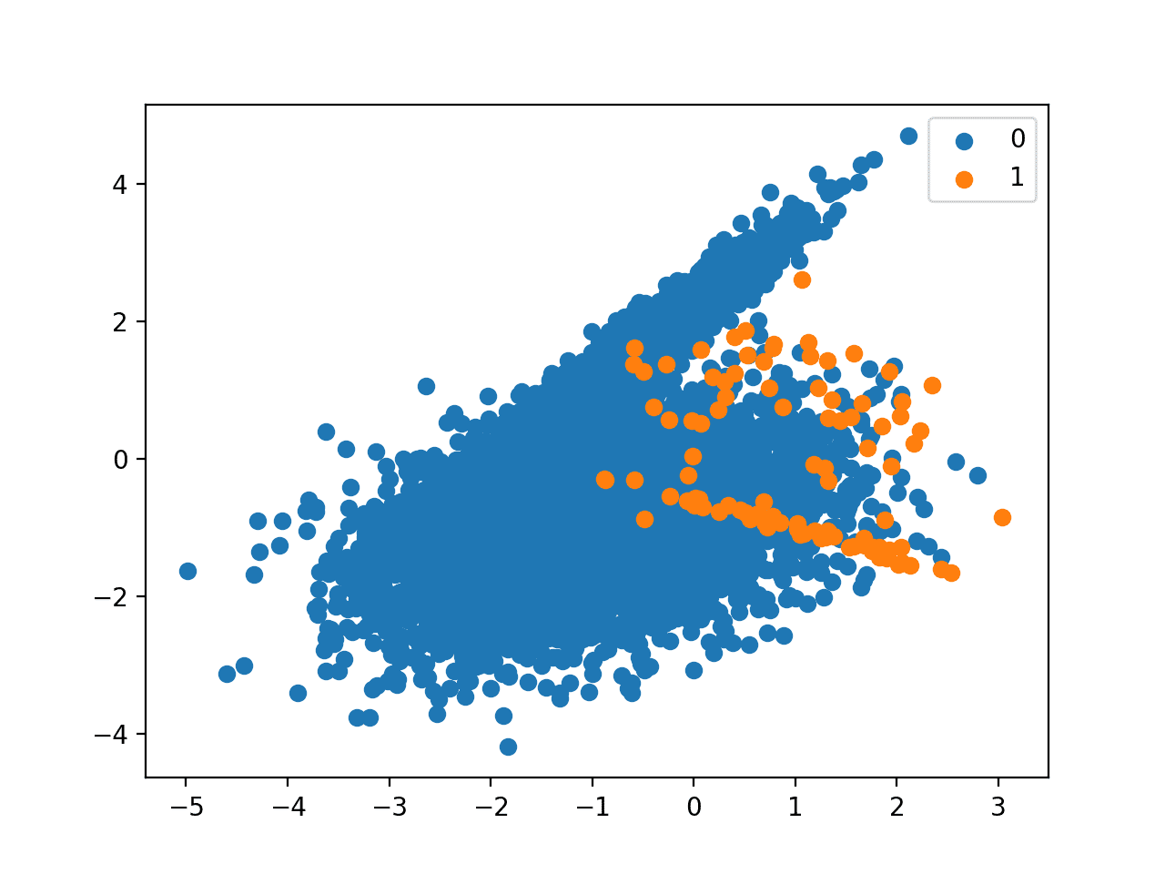
Finally, we can create a scatter plot of the examples and color them by class label to help understand the challenge of classifying examples from this dataset.
Running the example first creates the dataset and summarizes the class distribution.
We can see that the dataset has an approximate 1:100 class distribution with a little less than 10,000 examples in the majority class and 100 in the minority class.
1
Counter({0: 9900, 1: 100})
Next, a scatter plot of the dataset is created showing the large mass of examples for the majority class (blue) and a small number of examples for the minority class (orange), with some modest class overlap.
Scatter Plot of Binary Classification Dataset With 1 to 100 Class Imbalance
Want to Get Started With Imbalance Classification?
Take my free 7-day email crash course now (with sample code).
Click to sign-up and also get a free PDF Ebook version of the course.
XGBoost Model for Classification
XGBoost is short for Extreme Gradient Boosting and is an efficient implementation of the stochastic gradient boosting machine learning algorithm.
The stochastic gradient boosting algorithm, also called gradient boosting machines or tree boosting, is a powerful machine learning technique that performs well or even best on a wide range of challenging machine learning problems.
Tree boosting has been shown to give state-of-the-art results on many standard classification benchmarks.
It is an ensemble of decision trees algorithm where new trees fix errors of those trees that are already part of the model. Trees are added until no further improvements can be made to the model.
XGBoost provides a highly efficient implementation of the stochastic gradient boosting algorithm and access to a suite of model hyperparameters designed to provide control over the model training process.
The most important factor behind the success of XGBoost is its scalability in all scenarios. The system runs more than ten times faster than existing popular solutions on a single machine and scales to billions of examples in distributed or memory-limited settings.
XGBoost is an effective machine learning model, even on datasets where the class distribution is skewed.
Before any modification or tuning is made to the XGBoost algorithm for imbalanced classification, it is important to test the default XGBoost model and establish a baseline in performance.
Although the XGBoost library has its own Python API, we can use XGBoost models with the scikit-learn API via the XGBClassifier wrapper class. An instance of the model can be instantiated and used just like any other scikit-learn class for model evaluation. For example:
1
2
3
...
# define model
model=XGBClassifier()
We will use repeated cross-validation to evaluate the model, with three repeats of 10-fold cross-validation.
The model performance will be reported using the mean ROC area under curve (ROC AUC) averaged over repeats and all folds.
Running the example evaluates the default XGBoost model on the imbalanced dataset and reports the mean ROC AUC.
Note: Your results may vary given the stochastic nature of the algorithm or evaluation procedure, or differences in numerical precision. Consider running the example a few times and compare the average outcome.
We can see that the model has skill, achieving a ROC AUC above 0.5, in this case achieving a mean score of 0.95724.
1
Mean ROC AUC: 0.95724
This provides a baseline for comparison for any hyperparameter tuning performed for the default XGBoost algorithm.
Weighted XGBoost for Class Imbalance
Although the XGBoost algorithm performs well for a wide range of challenging problems, it offers a large number of hyperparameters, many of which require tuning in order to get the most out of the algorithm on a given dataset.
The implementation provides a hyperparameter designed to tune the behavior of the algorithm for imbalanced classification problems; this is the scale_pos_weight hyperparameter.
By default, the scale_pos_weight hyperparameter is set to the value of 1.0 and has the effect of weighing the balance of positive examples, relative to negative examples when boosting decision trees. For an imbalanced binary classification dataset, the negative class refers to the majority class (class 0) and the positive class refers to the minority class (class 1).
XGBoost is trained to minimize a loss function and the “gradient” in gradient boosting refers to the steepness of this loss function, e.g. the amount of error. A small gradient means a small error and, in turn, a small change to the model to correct the error. A large error gradient during training in turn results in a large correction.
Small Gradient: Small error or correction to the model.
Large Gradient: Large error or correction to the model.
Gradients are used as the basis for fitting subsequent trees added to boost or correct errors made by the existing state of the ensemble of decision trees.
The scale_pos_weight value is used to scale the gradient for the positive class.
This has the effect of scaling errors made by the model during training on the positive class and encourages the model to over-correct them. In turn, this can help the model achieve better performance when making predictions on the positive class. Pushed too far, it may result in the model overfitting the positive class at the cost of worse performance on the negative class or both classes.
As such, the scale_pos_weight can be used to train a class-weighted or cost-sensitive version of XGBoost for imbalanced classification.
A sensible default value to set for the scale_pos_weight hyperparameter is the inverse of the class distribution. For example, for a dataset with a 1 to 100 ratio for examples in the minority to majority classes, the scale_pos_weight can be set to 100. This will give classification errors made by the model on the minority class (positive class) 100 times more impact, and in turn, 100 times more correction than errors made on the majority class.
For example:
1
2
3
...
# define model
model=XGBClassifier(scale_pos_weight=100)
The XGBoost documentation suggests a fast way to estimate this value using the training dataset as the total number of examples in the majority class divided by the total number of examples in the minority class.
For example, we can calculate this value for our synthetic classification dataset. We would expect this to be about 100, or more precisely, 99 given the weighting we used to define the dataset.
1
2
3
4
5
6
...
# count examples in each class
counter=Counter(y)
# estimate scale_pos_weight value
estimate=counter[0]/counter[1]
print('Estimate: %.3f'%estimate)
The complete example of estimating the value for the scale_pos_weight XGBoost hyperparameter is listed below.
1
2
3
4
5
6
7
8
9
10
11
# estimate a value for the scale_pos_weight xgboost hyperparameter
Running the example creates the dataset and estimates the values of the scale_pos_weight hyperparameter as 99, as we expected.
1
Estimate: 99.000
We will use this value directly in the configuration of the XGBoost model and evaluate its performance on the dataset using repeated k-fold cross-validation.
We would expect some improvement in ROC AUC, although this is not guaranteed depending on the difficulty of the dataset and the chosen configuration of the XGBoost model.
The complete example is listed below.
1
2
3
4
5
6
7
8
9
10
11
12
13
14
15
16
17
# fit balanced xgboost on an imbalanced classification dataset
from numpy import mean
from sklearn.datasets import make_classification
from sklearn.model_selection import cross_val_score
from sklearn.model_selection import RepeatedStratifiedKFold
Running the example prepares the synthetic imbalanced classification dataset, then evaluates the class-weighted version of the XGBoost training algorithm using repeated cross-validation.
Note: Your results may vary given the stochastic nature of the algorithm or evaluation procedure, or differences in numerical precision. Consider running the example a few times and compare the average outcome.
In this case, we can see a modest lift in performance from a ROC AUC of about 0.95724 with scale_pos_weight=1 in the previous section to a value of 0.95990 with scale_pos_weight=99.
1
Mean ROC AUC: 0.95990
Tune the Class Weighting Hyperparameter
The heuristic for setting the scale_pos_weight is effective for many situations.
Nevertheless, it is possible that better performance can be achieved with a different class weighting, and this too will depend on the choice of performance metric used to evaluate the model.
In this section, we will grid search a range of different class weightings for class-weighted XGBoost and discover which results in the best ROC AUC score.
We will try the following weightings for the positive class:
1 (default)
10
25
50
75
99 (recommended)
100
1000
These can be defined as grid search parameters for the GridSearchCV class as follows:
1
2
3
4
...
# define grid
weights=[1,10,25,50,75,99,100,1000]
param_grid=dict(scale_pos_weight=weights)
We can perform the grid search on these parameters using repeated cross-validation and estimate model performance using ROC AUC:
print("Best: %f using %s"%(grid_result.best_score_,grid_result.best_params_))
# report all configurations
means=grid_result.cv_results_['mean_test_score']
stds=grid_result.cv_results_['std_test_score']
params=grid_result.cv_results_['params']
formean,stdev,param inzip(means,stds,params):
print("%f (%f) with: %r"%(mean,stdev,param))
Running the example evaluates each positive class weighting using repeated k-fold cross-validation and reports the best configuration and the associated mean ROC AUC score.
Note: Your results may vary given the stochastic nature of the algorithm or evaluation procedure, or differences in numerical precision. Consider running the example a few times and compare the average outcome.
In this case, we can see that the scale_pos_weight=99 positive class weighting achieved the best mean ROC score. This matches the configuration for the general heuristic.
It’s interesting to note that almost all values larger than the default value of 1 have a better mean ROC AUC, even the aggressive value of 1,000. It’s also interesting to note that a value of 99 performed better from the value of 100, which I may have used if I did not calculate the heuristic as suggested in the XGBoost documentation.
It provides self-study tutorials and end-to-end projects on: Performance Metrics, Undersampling Methods, SMOTE, Threshold Moving, Probability Calibration, Cost-Sensitive Algorithms
and much more...
Bring Imbalanced Classification Methods to Your Machine Learning Projects
Can u say how to use F1 metric instead of auc in r? like in xgboost function there is one option for specifying eval_metric ; can u say what argument will be appropriate under eval_metric for F1 score?
Hello Jason,
I have a question about GridSearchCV.
What is the difference between GridSearchCV and RandomizedSearchCV?
Do you have an example of both?
Thanks
Thanks for the excellent tutorial!
I would like to know how to deal with multiclass classification
while Counter in the example can be used for binary, how to calculate/estimate the scale_pos_weight of my dataset?
# Since there is not class_weight option in XGBoost
# Use sample_weight to balance multi-class sizes by applying class weight to each data instance
# Calculate class weight
from sklearn.utils import class_weight
k_train = class_weight.compute_class_weight(‘balanced’, np.unique(y_train), y_train)
wt = dict(zip(np.unique(y_train), k_train))
# Map class weights to corresponding target class values, make sure class labels have range (0, n_classes-1)
w_array = y_train.map(wt)
set(zip(y_train,w_array))
# Convert wt series to wt array
w_array = w_array.values
#Apply wt array to .fit()
model.fit(X_train, y_train, eval_metric=’auc’, sample_weight=w_array)
My dataset is of shape – 5621*8 (binary classification)
– Label/targtet : Success (4324, 77 %) & Not success (1297, 23 %)
I split my data into 3 (Train, Validate, test)
– For train & Validate i perform 10 fold CV.
– Test is the seperate data, which I evaluate for each folds
I tune my scale_pos_weight ranging between 5 to 80, and Finally I fixed my values as 75 since I got average higher accuracy rate for my Test set (79 %) for those 10 folds
But, If i check my average auc_roc metrics it is very poor, i.e only 50 % for all 10 folds.
If i did not tune scale_pos_weight my avg.accuracy drops to 50% & my avg auc_roc increases to 70 %.
How can I interpret from the above results ?
What is the problem in my case?
Will all these articles and tutorial with each archive, such as here Imbalance Data archive, is contained in each respective of your book? For instance, all of the archive for Imbalance Data is in your book on Imbalance Data.
The reason I asked is that I just came across your webpage yesterday, and its a bit overwhelming for me. So, I wonder the question above making sure I can only rely on one source of information from you, i.e. book.
Where is my previous question??? So, the initial question is, will the blog you published here is the subset of your book? Will I miss something if I just refer to your book and not the blog here?
Thank you for this wonderful article. I used this method of adding weight for training my model.
Although I got better results with this, I noticed that the prediction probability has shifted a lot.
1. Can you please help me understand why the shift in prediction probability?
2. Is there any way to calculate the prediction probability as you would get without using these weights method?
Thank you for responding quickly.
I performed tuning and the model looks good. And I used predict_proba like you mentioned.
When I look at the prediction probability of a model with weights vs the prediction probability from the model without weight, I found that the value of the former to be higher.
When I tried searching for an explanation, I only find posts that say that yes there will be increase in the probability value and that we need to recalibrate them. But I dont find any helpful article that would explain why there is a shift in the prediction probability.
I am hoping you can help me understand this shift.
We usually compare the prediction vs actually using decile charts which uses prediction probability. My team had asked me questions on why the prediction probability is high and I wasnt able to give a good explanation. I found several articles of yours using these weighted models and I tried them all and almost all of them gave high prediction probabilities. Thats why I am hoping for an explanation from you.
Although the model is skillful I would like to understand more in depth regarding why these shifts happen.
In terms of XGBoost producing uncalibrated probabilities and how to calibrate them? Its something that I am hearing of for the first time so I dont have much knowledge on calibrating probabilities.
Thank you
I found this article very useful in understanding the concept and after using this I got better prediction probabilities.
I just have a basic question on when to know to calibrate probabilities? Is it based on the model types like Boosted models vs others or is it based on anything else?
I really want to thank you for these awesome articles and the time and effort you take to answer every question.
Specifically, any algorithm that does not natively predict probabilities should be calibrated. E.g. any decision tree or ensemble of decision tree algorithm.
I am using this model for an imbalanced dataset, but I am looking to produce accuracy, precision, re-call and f1 scores, as well as feature importance. Could please advise the code to use in combination with the current data imbalance code
So, using a class weight in this case increased the AUC from 0.9572 to 0.9599. That is less than one third of a percentage point.
Firstly, that size of an increase in AUC is not a material improvement in a classifier. To me I would describe it as no change in performance.
Secondly, as you said, this is a stochastic algorithm. I would bet that the variation in the AUC due to the stochastic nature of the algorithm would be greater than an increase of 0.00278.
It maybe the scenario is a poor showcase for the method. Nevertheless, the method is clearly presented so you can copy-paste and start using it in your project (the goal of the piece).
Okay cool. It’s always good to confirm that I’m understanding correctly! Have you encountered problems where using class weights improved the model? (I guess “improved” is relative, but what do you think?)
For imbalanced dataset, AUC-PR or average precision might be a better choice of metric, you might see a more interesting rise in scores than with AUC, that is already near 100%.
As far as I undrestood. The results are the accuracy of the training model and predicting the new data was not part of the code. How to increase the perfomance of the model to have accurate prediction on the test set?
I can confirm that your result is correct. Note that XGBoost changed a bit on its behavior (e.g., default to logloss instead of error) but also the scikit-learn that generated the data is depending on a random number generator. Hence you should never expect to see the exact result.
Every one of your eight ROC AUC values (for different scale_pos_weight) is *well* within its standard error of the mean (your parenthesized standard deviation / sqrt(10)) of their overall average of 0.959.
So your conclusion *should* be that the effects of of changing scale_pos_weight are statistically insignificant (completely consistent with being random fluctuations due to the variability in the random sampling inherent in the cross-validation, or in drawing your overall dataset from an underlying population for that matter).
In fact, your results merely confirm the fact that class-weighting (or simple over- or under-sampling for that matter) has no systematic effect whatsoever on classifier performance when the performance criterion is the ROC AUC, because the ROC, and thus its AUC, are inherently-independent of the class distribution or imbalance.


Shouldn’t you use a hold-out validation set for your grid search? Otherwise it seems like you’re overfitting your hyperparameters to your data.
Grid search uses cross-validation to estimate the performance of each config.
Ideally we would tune using a different hold out dataset. I typically don’t to keep the examples simple:
https://machinelearningmastery.com/faq/single-faq/why-do-you-use-the-test-dataset-as-the-validation-dataset
Why are you using AuC ROC if it’s imbalanced? The tpr will be high? Why not use precision, recall, f1?
ROC will still report a relative lift. Yes, those other metrics are great too.
See this framework for choosing a metric based on the goals of the project:
https://machinelearningmastery.com/tour-of-evaluation-metrics-for-imbalanced-classification/
Hi Jason,
When dealing with Imbalanced datasets, wouldn’t it be better to use another performance metric such as precision, recall or F1 instead of ROC-AUC?
Because 99% of cases belongs to class 0 and most of them are correctly classified, but may be not the minority class (1).
Thanks,
The focus of this post is on cost-sensitive xgboost.
For more on choosing an appropriate metric, see this:
https://machinelearningmastery.com/tour-of-evaluation-metrics-for-imbalanced-classification/
Can u say how to use F1 metric instead of auc in r? like in xgboost function there is one option for specifying eval_metric ; can u say what argument will be appropriate under eval_metric for F1 score?
Hi Saikat…The following resource may be of interest to you:
https://stats.stackexchange.com/questions/138690/calculate-the-f1-score-of-precision-and-recall-in-r
Hello Jason,
I have a question about GridSearchCV.
What is the difference between GridSearchCV and RandomizedSearchCV?
Do you have an example of both?
Thanks
Searching a specified grid of configs vs searching random combinations of configs.
Hey, thanks for the awesome article.
How do we set “scale_pos_weight” for mutli-class problems?
Thanks so much
I don’t think you can. I think it is for binary classification only.
Thanks for the excellent tutorial!
I would like to know how to deal with multiclass classification
while Counter in the example can be used for binary, how to calculate/estimate the scale_pos_weight of my dataset?
You’re welcome.
I don’t believe the approach that xgboost uses for imbalanced classification supports multiple classes.
I apply weight to each data instance:
# Since there is not class_weight option in XGBoost
# Use sample_weight to balance multi-class sizes by applying class weight to each data instance
# Calculate class weight
from sklearn.utils import class_weight
k_train = class_weight.compute_class_weight(‘balanced’, np.unique(y_train), y_train)
wt = dict(zip(np.unique(y_train), k_train))
# Map class weights to corresponding target class values, make sure class labels have range (0, n_classes-1)
w_array = y_train.map(wt)
set(zip(y_train,w_array))
# Convert wt series to wt array
w_array = w_array.values
#Apply wt array to .fit()
model.fit(X_train, y_train, eval_metric=’auc’, sample_weight=w_array)
Dear Sir,
I want to know how I can use my dataset in place of
X, y = make_classification(n_samples=10000, n_features=2, n_redundant=0,
n_clusters_per_class=2, weights=[0.99], flip_y=0, random_state=7)
Load your data as a numpy array:
https://machinelearningmastery.com/load-machine-learning-data-python/
Hallo Jason,
Thanks for your excellent article.
My dataset is of shape – 5621*8 (binary classification)
– Label/targtet : Success (4324, 77 %) & Not success (1297, 23 %)
I split my data into 3 (Train, Validate, test)
– For train & Validate i perform 10 fold CV.
– Test is the seperate data, which I evaluate for each folds
I tune my scale_pos_weight ranging between 5 to 80, and Finally I fixed my values as 75 since I got average higher accuracy rate for my Test set (79 %) for those 10 folds
But, If i check my average auc_roc metrics it is very poor, i.e only 50 % for all 10 folds.
If i did not tune scale_pos_weight my avg.accuracy drops to 50% & my avg auc_roc increases to 70 %.
How can I interpret from the above results ?
What is the problem in my case?
Waiting for your reply-
Perhaps the model is not appropriate for your dataset and chosen metric, perhaps try other methods?
Hi Jason,
Will all these articles and tutorial with each archive, such as here Imbalance Data archive, is contained in each respective of your book? For instance, all of the archive for Imbalance Data is in your book on Imbalance Data.
Some are early versions of chapters of the book, some are not.
You can see the full table of contents for the book here:
https://machinelearningmastery.com/imbalanced-classification-with-python/
Will I miss something if I just refer to your book and not the blog? or if l the blog is the subset of the book?
The best tutorials are in the books. I spend a long time carefully designing, editing, and testing the book tutorials with my team of editors.
The blog might be a useful complement in some cases.
The reason I asked is that I just came across your webpage yesterday, and its a bit overwhelming for me. So, I wonder the question above making sure I can only rely on one source of information from you, i.e. book.
Where is my previous question??? So, the initial question is, will the blog you published here is the subset of your book? Will I miss something if I just refer to your book and not the blog here?
Comments must be reviewed and approved by me, it can take a while sometimes as I work through them in batches:
https://machinelearningmastery.com/faq/single-faq/where-is-my-blog-comment
The books are the best source of my knowledge/ideas.
This might be an easier place to start:
https://machinelearningmastery.com/start-here/
how do i use
scale_pos_weightfor multi-class problems?I don’t think it supports multi-class problems.
Hi! if I do gridsearch on training set, should I find the estimate for scale_pos_weight value on training set (y_train) or on all y-s? I mean this
# count examples in each class
counter = Counter(y)
# estimate scale_pos_weight value
estimate = counter[0] / counter[1]
print(‘Estimate: %.3f’ % estimate)
Yes, but it might be case of data leakage.
Ideally, we would set the weight based on the training set only.
Thank you for this wonderful article. I used this method of adding weight for training my model.
Although I got better results with this, I noticed that the prediction probability has shifted a lot.
1. Can you please help me understand why the shift in prediction probability?
2. Is there any way to calculate the prediction probability as you would get without using these weights method?
Perhaps the model requires further tuning on your problem?
Perhaps you can try calibrating the probabilities predicted by the model?
You can predict probabilities via a call to
Hi,
Thank you for responding quickly.
I performed tuning and the model looks good. And I used predict_proba like you mentioned.
When I look at the prediction probability of a model with weights vs the prediction probability from the model without weight, I found that the value of the former to be higher.
When I tried searching for an explanation, I only find posts that say that yes there will be increase in the probability value and that we need to recalibrate them. But I dont find any helpful article that would explain why there is a shift in the prediction probability.
I am hoping you can help me understand this shift.
Thanks
Does the “why” matter?
We seek a skilful model, even if the model is opaque, which many are, it is the skilful predictions that matter more than model interpretation:
https://machinelearningmastery.com/faq/single-faq/how-do-i-interpret-the-predictions-from-my-model
Hi,
We usually compare the prediction vs actually using decile charts which uses prediction probability. My team had asked me questions on why the prediction probability is high and I wasnt able to give a good explanation. I found several articles of yours using these weighted models and I tried them all and almost all of them gave high prediction probabilities. Thats why I am hoping for an explanation from you.
Although the model is skillful I would like to understand more in depth regarding why these shifts happen.
Generally xgboost models product uncalibrated probabilities as far as I recall. The confidence of the predictions is probably arbitrary.
I strongly recommend calibrating probabilities before interpreting them.
Can you please explain this more?
Thank you
No problem, which part is confusing?
In terms of XGBoost producing uncalibrated probabilities and how to calibrate them? Its something that I am hearing of for the first time so I dont have much knowledge on calibrating probabilities.
Thank you
This tutorial will show you how:
https://machinelearningmastery.com/calibrated-classification-model-in-scikit-learn/
Hi
I found another article of yours about calibrating probabilities,
https://machinelearningmastery.com/calibrated-classification-model-in-scikit-learn/
I found this article very useful in understanding the concept and after using this I got better prediction probabilities.
I just have a basic question on when to know to calibrate probabilities? Is it based on the model types like Boosted models vs others or is it based on anything else?
I really want to thank you for these awesome articles and the time and effort you take to answer every question.
Generally, try it and see.
Specifically, any algorithm that does not natively predict probabilities should be calibrated. E.g. any decision tree or ensemble of decision tree algorithm.
Hello,
I am using this model for an imbalanced dataset, but I am looking to produce accuracy, precision, re-call and f1 scores, as well as feature importance. Could please advise the code to use in combination with the current data imbalance code
Thank you
I recommend choosing one metric to optimize, and accuracy is typically a poor metric for imbalanced data.
This will help you choose a metric:
https://machinelearningmastery.com/tour-of-evaluation-metrics-for-imbalanced-classification/
So, using a class weight in this case increased the AUC from 0.9572 to 0.9599. That is less than one third of a percentage point.
Firstly, that size of an increase in AUC is not a material improvement in a classifier. To me I would describe it as no change in performance.
Secondly, as you said, this is a stochastic algorithm. I would bet that the variation in the AUC due to the stochastic nature of the algorithm would be greater than an increase of 0.00278.
Maybe I’m missing something?
Agreed.
It maybe the scenario is a poor showcase for the method. Nevertheless, the method is clearly presented so you can copy-paste and start using it in your project (the goal of the piece).
Okay cool. It’s always good to confirm that I’m understanding correctly! Have you encountered problems where using class weights improved the model? (I guess “improved” is relative, but what do you think?)
Yes, I have a few case studies on the blog where using class weights/cost sensitive version of a model results in better performance.
For example, a cost-sensitive version of random forest gives best results here:
https://machinelearningmastery.com/imbalanced-multiclass-classification-with-the-glass-identification-dataset/
Ah, ok, thanks.
For imbalanced dataset, AUC-PR or average precision might be a better choice of metric, you might see a more interesting rise in scores than with AUC, that is already near 100%.
Agreed! See this:
https://machinelearningmastery.com/tour-of-evaluation-metrics-for-imbalanced-classification/
As far as I undrestood. The results are the accuracy of the training model and predicting the new data was not part of the code. How to increase the perfomance of the model to have accurate prediction on the test set?
To improve the performance of test set, you use cross validation techniques to calibrate your model.
I have xgboost version 1.5.0, but i got different result. The best score is when the scale_pos_weight is 1. Which xgboost version do you install?
I’m not sure what is the problem
Best: 0.960522 using {‘scale_pos_weight’: 1}
0.960522 (0.024031) with: {‘scale_pos_weight’: 1}
0.956106 (0.029382) with: {‘scale_pos_weight’: 10}
0.955189 (0.029265) with: {‘scale_pos_weight’: 25}
0.952980 (0.028971) with: {‘scale_pos_weight’: 50}
0.951190 (0.031723) with: {‘scale_pos_weight’: 75}
0.954692 (0.027654) with: {‘scale_pos_weight’: 99}
0.953470 (0.028217) with: {‘scale_pos_weight’: 100}
0.947552 (0.029872) with: {‘scale_pos_weight’: 1000}
I can confirm that your result is correct. Note that XGBoost changed a bit on its behavior (e.g., default to logloss instead of error) but also the scikit-learn that generated the data is depending on a random number generator. Hence you should never expect to see the exact result.
Hi Jason,
Every one of your eight ROC AUC values (for different scale_pos_weight) is *well* within its standard error of the mean (your parenthesized standard deviation / sqrt(10)) of their overall average of 0.959.
So your conclusion *should* be that the effects of of changing scale_pos_weight are statistically insignificant (completely consistent with being random fluctuations due to the variability in the random sampling inherent in the cross-validation, or in drawing your overall dataset from an underlying population for that matter).
In fact, your results merely confirm the fact that class-weighting (or simple over- or under-sampling for that matter) has no systematic effect whatsoever on classifier performance when the performance criterion is the ROC AUC, because the ROC, and thus its AUC, are inherently-independent of the class distribution or imbalance.