The OpenCV library has a module that implements the k-Nearest Neighbors algorithm for machine learning applications.
In this tutorial, you will learn how to apply OpenCV’s k-Nearest Neighbors algorithm for classifying handwritten digits.
After completing this tutorial, you will know:
- Several of the most important characteristics of the k-Nearest Neighbors algorithm.
- How to use the k-Nearest Neighbors algorithm for image classification in OpenCV.
Kick-start your project with my book Machine Learning in OpenCV. It provides self-study tutorials with working code.
Let’s get started.

K-Nearest Neighbors Classification Using OpenCV
Photo by Gleren Meneghin, some rights reserved.
Tutorial Overview
This tutorial is divided into two parts; they are:
- Reminder of How the k-Nearest Neighbors Algorithm Works
- Using k-Nearest Neighbors for Image Classification in OpenCV
Prerequisites
For this tutorial, we assume that you are already familiar with:
Reminder of How the k-Nearest Neighbors Algorithm Works
The k-Nearest Neighbors (kNN) algorithm has already been explained well in this tutorial by Jason Brownlee, but let’s first start with brushing up on some of the most important points from his tutorial:
- The kNN algorithm does not involve any learning. It simply stores and uses the entire training dataset as its model representation. For this reason, kNN is also called a lazy learning algorithm.
- Since the entire training dataset is stored, it would make sense to keep it curated, updated often with new data, and as free as possible from outliers.
- A new instance is predicted by searching the entire training dataset for the most similar instance based on a distance measure of choice. The choice of distance measure is typically based on the properties of the data.
- If the kNN is used to solve a regression problem, then the mean or the median of the k-most similar instances is typically used to generate a prediction.
- If the kNN is used to solve a classification problem, a prediction can be generated from the class with the highest frequency of k-most similar instances.
- A value for k can be tuned by trying out different values and seeing what works best for the problem.
- The kNN algorithm’s computational cost increases with the training dataset’s size. The kNN algorithm also struggles as the dimensionality of the input data increases.
Using k-Nearest Neighbors for Image Classification in OpenCV
In this tutorial, we will be considering the application of classifying handwritten digits.
In a previous tutorial, we have seen that OpenCV provides the image, digits.png, composed of a ‘collage’ of 5,000 sub-images in $20\times 20$ pixels, where each sub-image features a handwritten digit from 0 to 9.
We have also seen how to convert dataset images into feature vector representations before feeding them into a machine learning algorithm.
We shall be splitting OpenCV’s digits dataset into training and testing sets, converting them into feature vectors, and then using these feature vectors to train and test a kNN classifier to classify handwritten digits.
Note: We have previously mentioned that the kNN algorithm does not involve any training/learning, but we shall be referring to a training dataset to distinguish the images that will be used for the model representation from those that will be later used for testing.
Let’s start by loading OpenCV’s digits image, splitting it into training and testing sets of images, and converting them into feature vectors using the Histogram of Oriented Gradients (HOG) technique:
|
1 2 3 4 5 6 7 8 9 10 11 12 13 14 15 16 17 18 19 20 21 |
from cv2 import imshow, waitKey from digits_dataset import split_images, split_data from feature_extraction import hog_descriptors # Load the full training image img, sub_imgs = split_images('Images/digits.png', 20) # Check that the correct image has been loaded imshow('Training image', img) waitKey(0) # Check that the sub-images have been correctly split imshow('Sub-image', sub_imgs[0, 0, :, :].reshape(20, 20)) waitKey(0) # Split the dataset into training and testing train_imgs, train_labels, test_imgs, test_labels = split_data(20, sub_imgs, 0.5) # Convert the training and testing images into feature vectors using the HOG technique train_hog = hog_descriptors(train_imgs) test_hog = hog_descriptors(test_imgs) |
Next, we’re going to initiate a kNN classifier:
|
1 2 3 |
from cv2 import ml knn = ml.KNearest_create() |
Then ‘train’ it on the training split of the dataset. For the training split of the dataset, we may either use the intensity values of the image pixels themselves (type casted to 32-bit floating-point values, according to the expected input of the function):
|
1 |
knn.train(float32(train_imgs), ml.ROW_SAMPLE, train_labels) |
Or use the feature vectors generated by the HOG technique. In the previous section, we mentioned that the kNN algorithm struggles with high-dimensional data. Using the HOG technique to generate a more compact representation of the image data helps with alleviating this problem:
|
1 |
knn.train(train_hog, ml.ROW_SAMPLE, train_labels) |
Let’s continue this tutorial by making use of the HOG feature vectors.
The trained kNN classifier can now be tested on the testing split of the dataset, following which its accuracy can be computed by working out the percentage of correct predictions that match the ground truth. For the time being, the value for k will be empirically set to 3:
|
1 2 3 4 5 6 |
from numpy import sum k = 3 ret, result, neighbours, dist = knn.findNearest(test_hog, k) accuracy = (sum(result == test_labels) / test_labels.size) * 100 |
However, as we have mentioned in the previous section, it is typical practice that the value of k is tuned by trying out different values and seeing what works best for the problem at hand. We can also try splitting the dataset using different ratio values to see their effect on prediction accuracy.
To do so, we’ll place the kNN classifier code above into a nested for loop, where the outer loop iterates over different ratio values, whereas the inner loop iterates over different values of k. Inside the inner loop, we shall also populate a dictionary with the computed accuracy values to plot them later using Matplotlib.
One last detail that we will include is a check to ensure that we are loading the correct image and correctly splitting it into sub-images. For this purpose, we’ll make use of OpenCV’s imshow method to display the images, followed by a waitKey with an input of zero that will stop and wait for a keyboard event:
|
1 2 3 4 5 6 7 8 9 10 11 12 13 14 15 16 17 18 19 20 21 22 23 24 25 26 27 28 29 30 31 32 33 34 35 36 37 38 39 40 41 42 43 44 45 46 47 48 49 50 51 52 53 54 55 56 57 58 59 |
from cv2 import imshow, waitKey, ml from numpy import sum from matplotlib.pyplot import plot, show, title, xlabel, ylabel, legend from digits_dataset import split_images, split_data from feature_extraction import hog_descriptors # Load the full training image img, sub_imgs = split_images('Images/digits.png', 20) # Check that the correct image has been loaded imshow('Training image', img) waitKey(0) # Check that the sub-images have been correctly split imshow('Sub-image', sub_imgs[0, 0, :, :].reshape(20, 20)) waitKey(0) # Define different training-testing splits ratio = [0.5, 0.7, 0.9] for i in ratio: # Split the dataset into training and testing train_imgs, train_labels, test_imgs, test_labels = split_data(20, sub_imgs, i) # Convert the training and testing images into feature vectors using the HOG technique train_hog = hog_descriptors(train_imgs) test_hog = hog_descriptors(test_imgs) # Initiate a kNN classifier and train it on the training data knn = ml.KNearest_create() knn.train(train_hog, ml.ROW_SAMPLE, train_labels) # Initiate a dictionary to hold the ratio and accuracy values accuracy_dict = {} # Populate the dictionary with the keys corresponding to the values of 'k' keys = range(3, 16) for k in keys: # Test the kNN classifier on the testing data ret, result, neighbours, dist = knn.findNearest(test_hog, k) # Compute the accuracy and print it accuracy = (sum(result == test_labels) / test_labels.size) * 100 print("Accuracy: {0:.2f}%, Training: {1:.0f}%, k: {2}".format(accuracy, i*100, k)) # Populate the dictionary with the values corresponding to the accuracy accuracy_dict[k] = accuracy # Plot the accuracy values against the value of 'k' plot(accuracy_dict.keys(), accuracy_dict.values(), marker='o', label=str(i * 100) + '%') title('Accuracy of the k-nearest neighbors model') xlabel('k') ylabel('Accuracy') legend(loc='upper right') show() |
Plotting the computed prediction accuracy for different ratio values and different values of k, gives a better insight into the effect that these different values have on the prediction accuracy for this particular application:
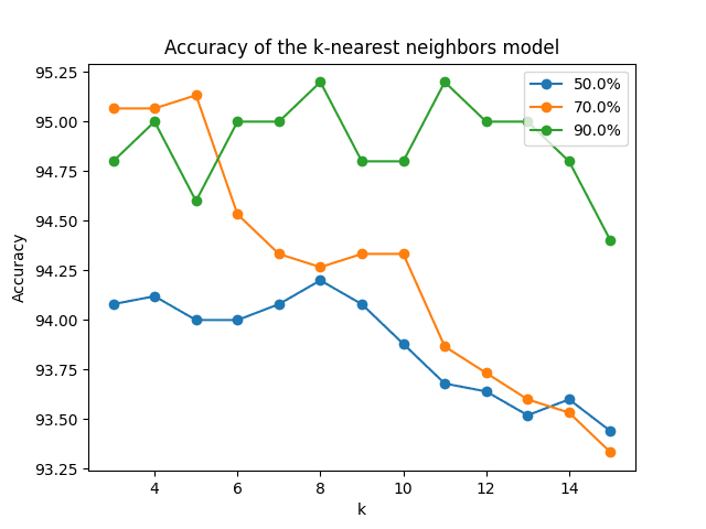
Line plots of the prediction accuracy for different training splits of the dataset, and different values of ‘k’
Try using different image descriptors and tweaking the different parameters for the algorithms of choice before feeding the data into the kNN algorithm, and investigate the kNN’s outputs that result from your changes.
Want to Get Started With Machine Learning with OpenCV?
Take my free email crash course now (with sample code).
Click to sign-up and also get a free PDF Ebook version of the course.
Further Reading
This section provides more resources on the topic if you want to go deeper.
Books
Websites
- OpenCV, https://opencv.org/
- OpenCV KNearest Class, https://docs.opencv.org/4.7.0/dd/de1/classcv_1_1ml_1_1KNearest.html
Summary
In this tutorial, you learned how to apply OpenCV’s k-Nearest Neighbors algorithm to classify handwritten digits.
Specifically, you learned:
- Several of the most important characteristics of the k-Nearest Neighbors algorithm.
- How to use the k-Nearest Neighbors algorithm for image classification in OpenCV.
Do you have any questions?
Ask your questions in the comments below, and I will do my best to answer.
Get Started on Machine Learning in OpenCV!
Learn how to use machine learning techniques in image processing projects
...using OpenCV in advanced ways and work beyond pixels
Discover how in my new Ebook:
Machine Learing in OpenCV
It provides self-study tutorials with all working code in Python to turn you from a novice to expert. It equips you with
logistic regression, random forest, SVM, k-means clustering, neural networks,
and much more...all using the machine learning module in OpenCV


No comments yet.