Nearest Centroids is a linear classification machine learning algorithm.
It involves predicting a class label for new examples based on which class-based centroid the example is closest to from the training dataset.
The Nearest Shrunken Centroids algorithm is an extension that involves shifting class-based centroids toward the centroid of the entire training dataset and removing those input variables that are less useful at discriminating the classes.
As such, the Nearest Shrunken Centroids algorithm performs an automatic form of feature selection, making it appropriate for datasets with very large numbers of input variables.
In this tutorial, you will discover the Nearest Shrunken Centroids classification machine learning algorithm.
After completing this tutorial, you will know:
- The Nearest Shrunken Centroids is a simple linear machine learning algorithm for classification.
- How to fit, evaluate, and make predictions with the Nearest Shrunken Centroids model with Scikit-Learn.
- How to tune the hyperparameters of the Nearest Shrunken Centroids algorithm on a given dataset.
Let’s get started.

Nearest Shrunken Centroids With Python
Photo by Giuseppe Milo, some rights reserved.
Tutorial Overview
This tutorial is divided into three parts; they are:
- Nearest Centroids Algorithm
- Nearest Centroids With Scikit-Learn
- Tuning Nearest Centroid Hyperparameters
Nearest Centroids Algorithm
Nearest Centroids is a classification machine learning algorithm.
The algorithm involves first summarizing the training dataset into a set of centroids (centers), then using the centroids to make predictions for new examples.
For each class, the centroid of the data is found by taking the average value of each predictor (per class) in the training set. The overall centroid is computed using the data from all of the classes.
— Page 307, Applied Predictive Modeling, 2013.
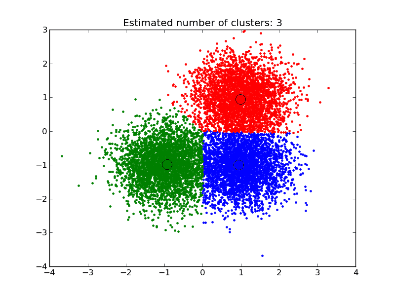
A centroid is the geometric center of a data distribution, such as the mean. In multiple dimensions, this would be the mean value along each dimension, forming a point of center of the distribution across each variable.
The Nearest Centroids algorithm assumes that the centroids in the input feature space are different for each target label. The training data is split into groups by class label, then the centroid for each group of data is calculated. Each centroid is simply the mean value of each of the input variables. If there are two classes, then two centroids or points are calculated; three classes give three centroids, and so on.
The centroids then represent the “model.” Given new examples, such as those in the test set or new data, the distance between a given row of data and each centroid is calculated and the closest centroid is used to assign a class label to the example.
Distance measures, such as Euclidean distance, are used for numerical data or hamming distance for categorical data, in which case it is best practice to scale input variables via normalization or standardization prior to training the model. This is to ensure that input variables with large values don’t dominate the distance calculation.
An extension to the nearest centroid method for classification is to shrink the centroids of each input variable towards the centroid of the entire training dataset. Those variables that are shrunk down to the value of the data centroid can then be removed as they do not help to discriminate between the class labels.
As such, the amount of shrinkage applied to the centroids is a hyperparameter that can be tuned for the dataset and used to perform an automatic form of feature selection. Thus, it is appropriate for a dataset with a large number of input variables, some of which may be irrelevant or noisy.
Consequently, the nearest shrunken centroid model also conducts feature selection during the model training process.
— Page 307, Applied Predictive Modeling, 2013.
This approach is referred to as “Nearest Shrunken Centroids” and was first described by Robert Tibshirani, et al. in their 2002 paper titled “Diagnosis Of Multiple Cancer Types By Shrunken Centroids Of Gene Expression.”
Nearest Centroids With Scikit-Learn
The Nearest Shrunken Centroids is available in the scikit-learn Python machine learning library via the NearestCentroid class.
The class allows the configuration of the distance metric used in the algorithm via the “metric” argument, which defaults to ‘euclidean‘ for the Euclidean distance metric.
This can be changed to other built-in metrics such as ‘manhattan.’
|
1 2 3 |
... # create the nearest centroid model model = NearestCentroid(metric='euclidean') |
By default, no shrinkage is used, but shrinkage can be specified via the “shrink_threshold” argument, which takes a floating point value between 0 and 1.
|
1 2 3 |
... # create the nearest centroid model model = NearestCentroid(metric='euclidean', shrink_threshold=0.5) |
We can demonstrate the Nearest Shrunken Centroids with a worked example.
First, let’s define a synthetic classification dataset.
We will use the make_classification() function to create a dataset with 1,000 examples, each with 20 input variables.
The example creates and summarizes the dataset.
|
1 2 3 4 5 6 |
# test classification dataset from sklearn.datasets import make_classification # define dataset X, y = make_classification(n_samples=1000, n_features=20, n_informative=15, n_redundant=5, random_state=1) # summarize the dataset print(X.shape, y.shape) |
Running the example creates the dataset and confirms the number of rows and columns of the dataset.
|
1 |
(1000, 20) (1000,) |
We can fit and evaluate a Nearest Shrunken Centroids model using repeated stratified k-fold cross-validation via the RepeatedStratifiedKFold class. We will use 10 folds and three repeats in the test harness.
We will use the default configuration of Euclidean distance and no shrinkage.
|
1 2 3 |
... # create the nearest centroid model model = NearestCentroid() |
The complete example of evaluating the Nearest Shrunken Centroids model for the synthetic binary classification task is listed below.
|
1 2 3 4 5 6 7 8 9 10 11 12 13 14 15 16 17 |
# evaluate an nearest centroid model on the dataset from numpy import mean from numpy import std from sklearn.datasets import make_classification from sklearn.model_selection import cross_val_score from sklearn.model_selection import RepeatedStratifiedKFold from sklearn.neighbors import NearestCentroid # define dataset X, y = make_classification(n_samples=1000, n_features=20, n_informative=15, n_redundant=5, random_state=1) # define model model = NearestCentroid() # define model evaluation method cv = RepeatedStratifiedKFold(n_splits=10, n_repeats=3, random_state=1) # evaluate model scores = cross_val_score(model, X, y, scoring='accuracy', cv=cv, n_jobs=-1) # summarize result print('Mean Accuracy: %.3f (%.3f)' % (mean(scores), std(scores))) |
Running the example evaluates the Nearest Shrunken Centroids algorithm on the synthetic dataset and reports the average accuracy across the three repeats of 10-fold cross-validation.
Your specific results may vary given the stochastic nature of the learning algorithm. Consider running the example a few times.
In this case, we can see that the model achieved a mean accuracy of about 71 percent.
|
1 |
Mean Accuracy: 0.711 (0.055) |
We may decide to use the Nearest Shrunken Centroids as our final model and make predictions on new data.
This can be achieved by fitting the model on all available data and calling the predict() function passing in a new row of data.
We can demonstrate this with a complete example listed below.
|
1 2 3 4 5 6 7 8 9 10 11 12 13 14 15 |
# make a prediction with a nearest centroid model on the dataset from sklearn.datasets import make_classification from sklearn.neighbors import NearestCentroid # define dataset X, y = make_classification(n_samples=1000, n_features=20, n_informative=15, n_redundant=5, random_state=1) # define model model = NearestCentroid() # fit model model.fit(X, y) # define new data row = [2.47475454,0.40165523,1.68081787,2.88940715,0.91704519,-3.07950644,4.39961206,0.72464273,-4.86563631,-6.06338084,-1.22209949,-0.4699618,1.01222748,-0.6899355,-0.53000581,6.86966784,-3.27211075,-6.59044146,-2.21290585,-3.139579] # make a prediction yhat = model.predict([row]) # summarize prediction print('Predicted Class: %d' % yhat) |
Running the example fits the model and makes a class label prediction for a new row of data.
|
1 |
Predicted Class: 0 |
Next, we can look at configuring the model hyperparameters.
Tuning Nearest Centroid Hyperparameters
The hyperparameters for the Nearest Shrunken Centroid method must be configured for your specific dataset.
Perhaps the most important hyperparameter is the shrinkage controlled via the “shrink_threshold” argument. It is a good idea to test values between 0 and 1 on a grid of values such as 0.1 or 0.01.
The example below demonstrates this using the GridSearchCV class with a grid of values we have defined.
|
1 2 3 4 5 6 7 8 9 10 11 12 13 14 15 16 17 18 19 20 21 22 |
# grid search shrinkage for nearest centroid from numpy import arange from sklearn.datasets import make_classification from sklearn.model_selection import GridSearchCV from sklearn.model_selection import RepeatedStratifiedKFold from sklearn.neighbors import NearestCentroid # define dataset X, y = make_classification(n_samples=1000, n_features=20, n_informative=15, n_redundant=5, random_state=1) # define model model = NearestCentroid() # define model evaluation method cv = RepeatedStratifiedKFold(n_splits=10, n_repeats=3, random_state=1) # define grid grid = dict() grid['shrink_threshold'] = arange(0, 1.01, 0.01) # define search search = GridSearchCV(model, grid, scoring='accuracy', cv=cv, n_jobs=-1) # perform the search results = search.fit(X, y) # summarize print('Mean Accuracy: %.3f' % results.best_score_) print('Config: %s' % results.best_params_) |
Running the example will evaluate each combination of configurations using repeated cross-validation.
Your specific results may vary given the stochastic nature of the learning algorithm. Try running the example a few times.
In this case, we can see that we achieved slightly better results than the default, with 71.4 percent vs 71.1 percent. We can see that the model assigned a shrink_threshold value of 0.53.
|
1 2 |
Mean Accuracy: 0.714 Config: {'shrink_threshold': 0.53} |
The other key configuration is the distance measure used, which can be chosen based on the distribution of the input variables.
Any of the built-in distance measures can be used, as listed here:
Common distance measures include:
- ‘cityblock’, ‘cosine’, ‘euclidean’, ‘l1’, ‘l2’, ‘manhattan’
For more on how these distance measures are calculated, see the tutorial:
Given that our input variables are numeric, our dataset only supports ‘euclidean‘ and ‘manhattan.’
We can include these metrics in our grid search; the complete example is listed below.
|
1 2 3 4 5 6 7 8 9 10 11 12 13 14 15 16 17 18 19 20 21 22 23 |
# grid search shrinkage and distance metric for nearest centroid from numpy import arange from sklearn.datasets import make_classification from sklearn.model_selection import GridSearchCV from sklearn.model_selection import RepeatedStratifiedKFold from sklearn.neighbors import NearestCentroid # define dataset X, y = make_classification(n_samples=1000, n_features=20, n_informative=15, n_redundant=5, random_state=1) # define model model = NearestCentroid() # define model evaluation method cv = RepeatedStratifiedKFold(n_splits=10, n_repeats=3, random_state=1) # define grid grid = dict() grid['shrink_threshold'] = arange(0, 1.01, 0.01) grid['metric'] = ['euclidean', 'manhattan'] # define search search = GridSearchCV(model, grid, scoring='accuracy', cv=cv, n_jobs=-1) # perform the search results = search.fit(X, y) # summarize print('Mean Accuracy: %.3f' % results.best_score_) print('Config: %s' % results.best_params_) |
Running the example fits the model and discovers the hyperparameters that give the best results using cross-validation.
Your specific results may vary given the stochastic nature of the learning algorithm. Try running the example a few times.
In this case, we can see that we get slightly better accuracy of 75 percent using no shrinkage and the manhattan instead of the euclidean distance measure.
|
1 2 |
Mean Accuracy: 0.750 Config: {'metric': 'manhattan', 'shrink_threshold': 0.0} |
A good extension to these experiments would be to add data normalization or standardization to the data as part of a modeling Pipeline.
Further Reading
This section provides more resources on the topic if you are looking to go deeper.
Tutorials
Papers
Books
APIs
Articles
Summary
In this tutorial, you discovered the Nearest Shrunken Centroids classification machine learning algorithm.
Specifically, you learned:
- The Nearest Shrunken Centroids is a simple linear machine learning algorithm for classification.
- How to fit, evaluate, and make predictions with the Nearest Shrunken Centroids model with Scikit-Learn.
- How to tune the hyperparameters of the Nearest Shrunken Centroids algorithm on a given dataset.
Do you have any questions?
Ask your questions in the comments below and I will do my best to answer.


Hi, How can we see the centroids of each dimension or feature and the main centroids of each target classes. Do you have any idea of creating a score for each entry
Via the “centroids_” property on the model:
https://scikit-learn.org/stable/modules/generated/sklearn.neighbors.NearestCentroid.html
Hi,
Thank you for the article. How do you change the define dataset line of code to input your own dataset of numbers (gene expression data).
Thank you
Hi Cameron…You may find the following helpful:
https://machinelearningmastery.com/how-to-load-data-in-python-with-scikit-learn/