Adding noise to an underconstrained neural network model with a small training dataset can have a regularizing effect and reduce overfitting.
Keras supports the addition of Gaussian noise via a separate layer called the GaussianNoise layer. This layer can be used to add noise to an existing model.
In this tutorial, you will discover how to add noise to deep learning models in Keras in order to reduce overfitting and improve model generalization.
After completing this tutorial, you will know:
- Noise can be added to a neural network model via the GaussianNoise layer.
- The GaussianNoise can be used to add noise to input values or between hidden layers.
- How to add a GaussianNoise layer in order to reduce overfitting in a Multilayer Perceptron model for classification.
Kick-start your project with my new book Better Deep Learning, including step-by-step tutorials and the Python source code files for all examples.
Let’s get started.
- Updated Oct/2019: Updated for Keras 2.3 and TensorFlow 2.0.

How to Improve Deep Learning Model Robustness by Adding Noise
Photo by Michael Mueller, some rights reserved.
Tutorial Overview
This tutorial is divided into three parts; they are:
- Noise Regularization in Keras
- Noise Regularization in Models
- Noise Regularization Case Study
Noise Regularization in Keras
Keras supports the addition of noise to models via the GaussianNoise layer.
This is a layer that will add noise to inputs of a given shape. The noise has a mean of zero and requires that a standard deviation of the noise be specified as a parameter. For example:
|
1 2 3 4 |
# import noise layer from keras.layers import GaussianNoise # define noise layer layer = GaussianNoise(0.1) |
The output of the layer will have the same shape as the input, with the only modification being the addition of noise to the values.
Noise Regularization in Models
The GaussianNoise can be used in a few different ways with a neural network model.
Firstly, it can be used as an input layer to add noise to input variables directly. This is the traditional use of noise as a regularization method in neural networks.
Below is an example of defining a GaussianNoise layer as an input layer for a model that takes 2 input variables.
|
1 2 3 |
... model.add(GaussianNoise(0.01, input_shape=(2,))) ... |
Noise can also be added between hidden layers in the model. Given the flexibility of Keras, the noise can be added before or after the use of the activation function. It may make more sense to add it before the activation; nevertheless, both options are possible.
Below is an example of a GaussianNoise layer that adds noise to the linear output of a Dense layer before a rectified linear activation function (ReLU), perhaps a more appropriate use of noise between hidden layers.
|
1 2 3 4 5 6 |
... model.add(Dense(32)) model.add(GaussianNoise(0.1)) model.add(Activation('relu')) model.add(Dense(32)) ... |
Noise can also be added after the activation function, much like using a noisy activation function. One downside of this usage is that the resulting values may be out-of-range from what the activation function may normally provide. For example, a value with added noise may be less than zero, whereas the relu activation function will only ever output values 0 or larger.
|
1 2 3 4 5 |
... model.add(Dense(32, activation='reu')) model.add(GaussianNoise(0.1)) model.add(Dense(32)) ... |
Let’s take a look at how noise regularization can be used with some common network types.
MLP Noise Regularization
The example below adds noise between two Dense fully connected layers.
|
1 2 3 4 5 6 7 8 9 10 |
# example of noise between fully connected layers from keras.layers import Dense from keras.layers import GaussianNoise from keras.layers import Activation ... model.add(Dense(32)) model.add(GaussianNoise(0.1)) model.add(Activation('relu')) model.add(Dense(1)) ... |
CNN Noise Regularization
The example below adds noise after a pooling layer in a convolutional network.
|
1 2 3 4 5 6 7 8 9 10 11 12 |
# example of noise for a CNN from keras.layers import Dense from keras.layers import Conv2D from keras.layers import MaxPooling2D from keras.layers import GaussianNoise ... model.add(Conv2D(32, (3,3))) model.add(Conv2D(32, (3,3))) model.add(MaxPooling2D()) model.add(GaussianNoise(0.1)) model.add(Dense(1)) ... |
RNN Dropout Regularization
The example below adds noise between an LSTM recurrent layer and a Dense fully connected layer.
|
1 2 3 4 5 6 7 8 9 10 11 |
# example of noise between LSTM and fully connected layers from keras.layers import Dense from keras.layers import Activation from keras.layers import LSTM from keras.layers import GaussianNoise ... model.add(LSTM(32)) model.add(GaussianNoise(0.5)) model.add(Activation('relu')) model.add(Dense(1)) ... |
Now that we have seen how to add noise to neural network models, let’s look at a case study of adding noise to an overfit model to reduce generalization error.
Want Better Results with Deep Learning?
Take my free 7-day email crash course now (with sample code).
Click to sign-up and also get a free PDF Ebook version of the course.
Noise Regularization Case Study
In this section, we will demonstrate how to use noise regularization to reduce overfitting of an MLP on a simple binary classification problem.
This example provides a template for applying noise regularization to your own neural network for classification and regression problems.
Binary Classification Problem
We will use a standard binary classification problem that defines two two-dimensional concentric circles of observations, one semi-circle for each class.
Each observation has two input variables with the same scale and a class output value of either 0 or 1. This dataset is called the “circles” dataset because of the shape of the observations in each class when plotted.
We can use the make_circles() function to generate observations from this problem. We will add noise to the data and seed the random number generator so that the same samples are generated each time the code is run.
|
1 2 |
# generate 2d classification dataset X, y = make_circles(n_samples=100, noise=0.1, random_state=1) |
We can plot the dataset where the two variables are taken as x and y coordinates on a graph and the class value is taken as the color of the observation.
The complete example of generating the dataset and plotting it is listed below.
|
1 2 3 4 5 6 7 8 9 10 11 12 13 14 |
# generate two circles dataset from sklearn.datasets import make_circles from matplotlib import pyplot from pandas import DataFrame # generate 2d classification dataset X, y = make_circles(n_samples=100, noise=0.1, random_state=1) # scatter plot, dots colored by class value df = DataFrame(dict(x=X[:,0], y=X[:,1], label=y)) colors = {0:'red', 1:'blue'} fig, ax = pyplot.subplots() grouped = df.groupby('label') for key, group in grouped: group.plot(ax=ax, kind='scatter', x='x', y='y', label=key, color=colors[key]) pyplot.show() |
Running the example creates a scatter plot showing the concentric circles shape of the observations in each class. We can see the noise in the dispersal of the points making the circles less obvious.
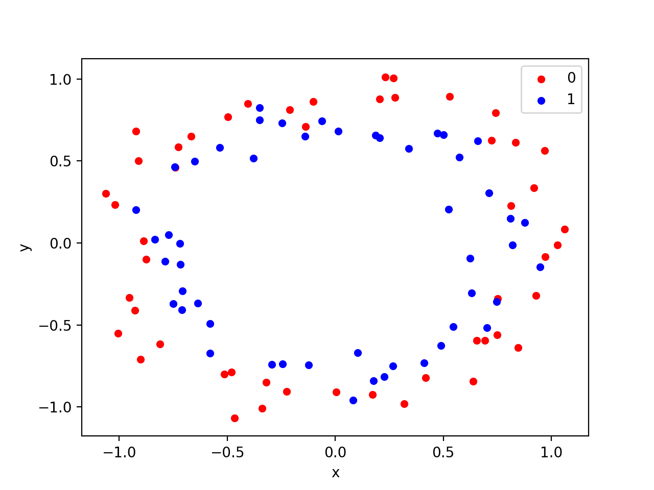
Scatter Plot of Circles Dataset with Color Showing the Class Value of Each Sample
This is a good test problem because the classes cannot be separated by a line, e.g. are not linearly separable, requiring a nonlinear method such as a neural network to address.
We have only generated 100 samples, which is small for a neural network, providing the opportunity to overfit the training dataset and have higher error on the test dataset, a good case for using regularization. Further, the samples have noise, giving the model an opportunity to learn aspects of the samples that don’t generalize.
Overfit Multilayer Perceptron
We can develop an MLP model to address this binary classification problem.
The model will have one hidden layer with more nodes than may be required to solve this problem, providing an opportunity to overfit. We will also train the model for longer than is required to ensure the model overfits.
Before we define the model, we will split the dataset into train and test sets, using 30 examples to train the model and 70 to evaluate the fit model’s performance.
|
1 2 3 4 5 6 |
# generate 2d classification dataset X, y = make_circles(n_samples=100, noise=0.1, random_state=1) # split into train and test n_train = 30 trainX, testX = X[:n_train, :], X[n_train:, :] trainy, testy = y[:n_train], y[n_train:] |
Next, we can define the model.
The hidden layer uses 500 nodes in the hidden layer and the rectified linear activation function. A sigmoid activation function is used in the output layer in order to predict class values of 0 or 1. The model is optimized using the binary cross entropy loss function, suitable for binary classification problems and the efficient Adam version of gradient descent.
|
1 2 3 4 5 |
# define model model = Sequential() model.add(Dense(500, input_dim=2, activation='relu')) model.add(Dense(1, activation='sigmoid')) model.compile(loss='binary_crossentropy', optimizer='adam', metrics=['accuracy']) |
The defined model is then fit on the training data for 4,000 epochs and the default batch size of 32.
We will also use the test dataset as a validation dataset.
|
1 2 |
# fit model history = model.fit(trainX, trainy, validation_data=(testX, testy), epochs=4000, verbose=0) |
We can evaluate the performance of the model on the test dataset and report the result.
|
1 2 3 4 |
# evaluate the model _, train_acc = model.evaluate(trainX, trainy, verbose=0) _, test_acc = model.evaluate(testX, testy, verbose=0) print('Train: %.3f, Test: %.3f' % (train_acc, test_acc)) |
Finally, we will plot the performance of the model on both the train and test set each epoch.
If the model does indeed overfit the training dataset, we would expect the line plot of accuracy on the training set to continue to increase and the test set to rise and then fall again as the model learns statistical noise in the training dataset.
|
1 2 3 4 5 |
# plot history pyplot.plot(history.history['accuracy'], label='train') pyplot.plot(history.history['val_accuracy'], label='test') pyplot.legend() pyplot.show() |
We can tie all of these pieces together; the complete example is listed below.
|
1 2 3 4 5 6 7 8 9 10 11 12 13 14 15 16 17 18 19 20 21 22 23 24 25 26 27 |
# mlp overfit on the two circles dataset from sklearn.datasets import make_circles from keras.layers import Dense from keras.models import Sequential from matplotlib import pyplot # generate 2d classification dataset X, y = make_circles(n_samples=100, noise=0.1, random_state=1) # split into train and test n_train = 30 trainX, testX = X[: n_train, :], X[n_train:, :] trainy, testy = y[:n_train], y[n_train:] # define model model = Sequential() model.add(Dense(500, input_dim=2, activation='relu')) model.add(Dense(1, activation='sigmoid')) model.compile(loss='binary_crossentropy', optimizer='adam', metrics=['accuracy']) # fit model history = model.fit(trainX, trainy, validation_data=(testX, testy), epochs=4000, verbose=0) # evaluate the model _, train_acc = model.evaluate(trainX, trainy, verbose=0) _, test_acc = model.evaluate(testX, testy, verbose=0) print('Train: %.3f, Test: %.3f' % (train_acc, test_acc)) # plot history pyplot.plot(history.history['accuracy'], label='train') pyplot.plot(history.history['val_accuracy'], label='test') pyplot.legend() pyplot.show() |
Running the example reports the model performance on the train and test datasets.
Note: Your results may vary given the stochastic nature of the algorithm or evaluation procedure, or differences in numerical precision. Consider running the example a few times and compare the average outcome.
We can see that the model has better performance on the training dataset than the test dataset, one possible sign of overfitting.
|
1 |
Train: 1.000, Test: 0.757 |
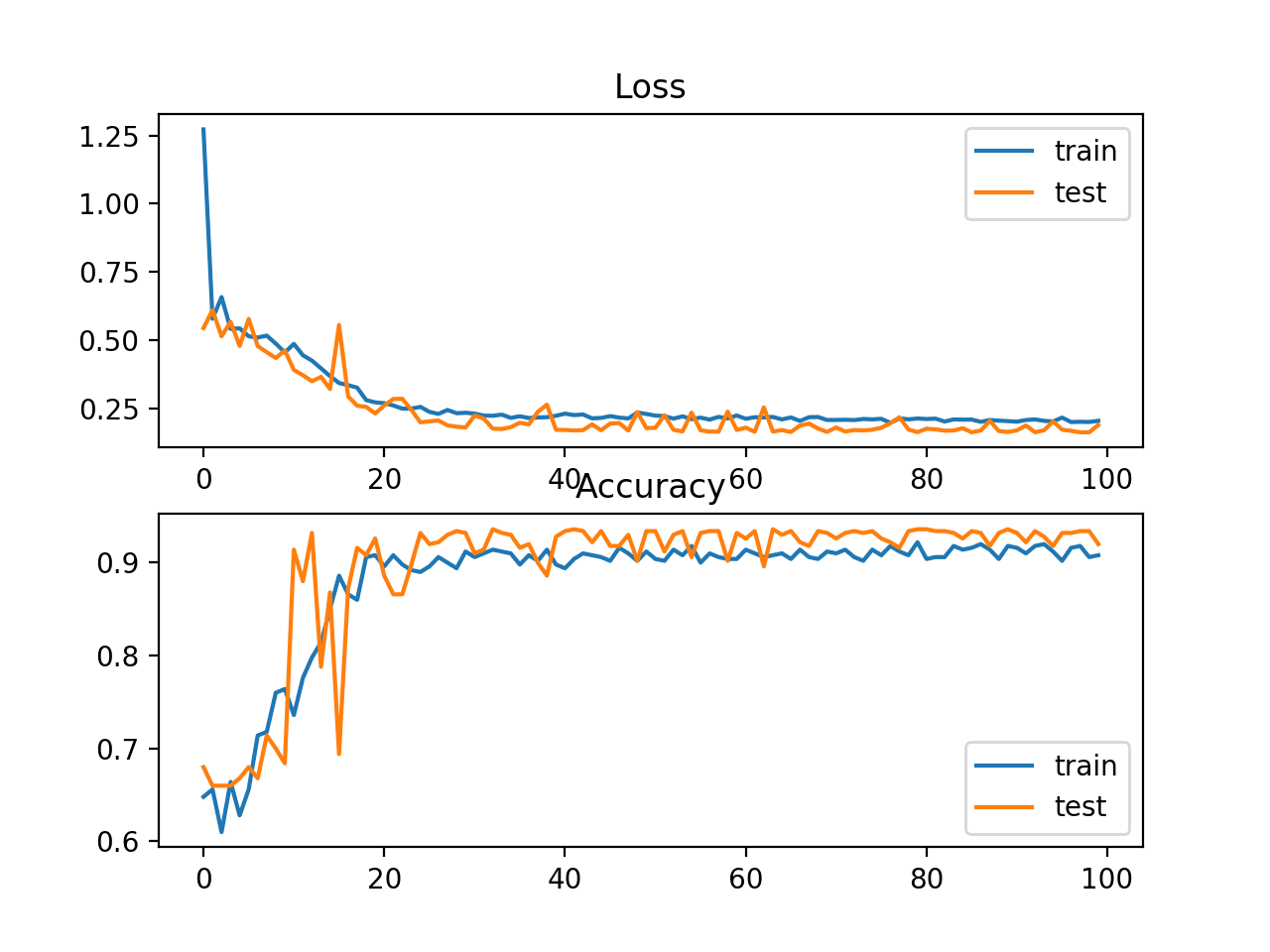
A figure is created showing line plots of the model accuracy on the train and test sets.
We can see that expected shape of an overfit model where test accuracy increases to a point and then begins to decrease again.
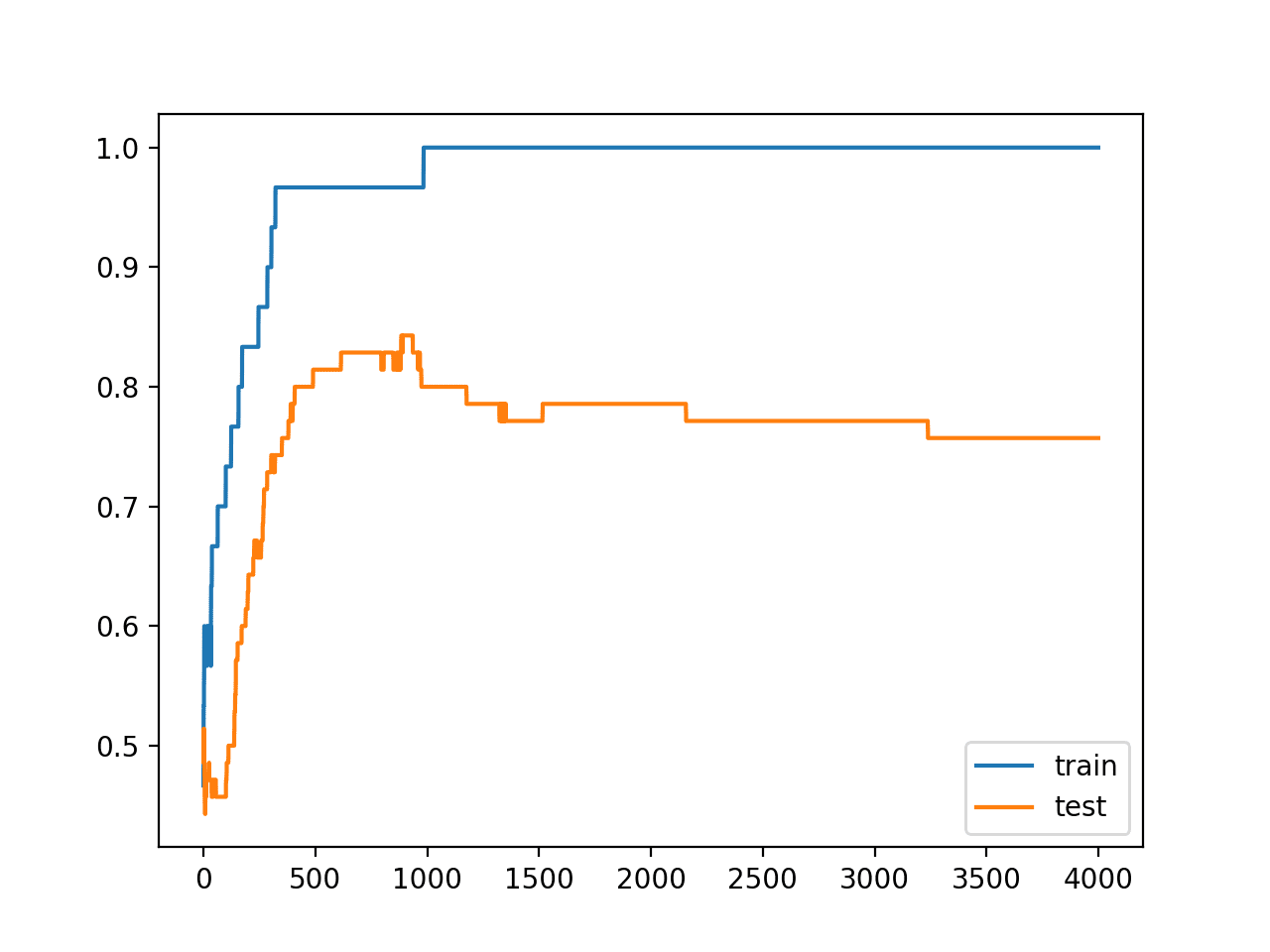
Line Plots of Accuracy on Train and Test Datasets While Training Showing an Overfit
MLP With Input Layer Noise
The dataset is defined by points that have a controlled amount of statistical noise.
Nevertheless, because the dataset is small, we can add further noise to the input values. This will have the effect of creating more samples or resampling the domain, making the structure of the input space artificially smoother. This may make the problem easier to learn and improve generalization performance.
We can add a GaussianNoise layer as the input layer. The amount of noise must be small. Given that the input values are within the range [0, 1], we will add Gaussian noise with a mean of 0.0 and a standard deviation of 0.01, chosen arbitrarily.
|
1 2 3 4 5 6 |
# define model model = Sequential() model.add(GaussianNoise(0.01, input_shape=(2,))) model.add(Dense(500, activation='relu')) model.add(Dense(1, activation='sigmoid')) model.compile(loss='binary_crossentropy', optimizer='adam', metrics=['accuracy']) |
The complete example with this change is listed below.
|
1 2 3 4 5 6 7 8 9 10 11 12 13 14 15 16 17 18 19 20 21 22 23 24 25 26 27 28 29 |
# mlp overfit on the two circles dataset with input noise from sklearn.datasets import make_circles from keras.models import Sequential from keras.layers import Dense from keras.layers import GaussianNoise from matplotlib import pyplot # generate 2d classification dataset X, y = make_circles(n_samples=100, noise=0.1, random_state=1) # split into train and test n_train = 30 trainX, testX = X[:n_train, :], X[n_train:, :] trainy, testy = y[:n_train], y[n_train:] # define model model = Sequential() model.add(GaussianNoise(0.01, input_shape=(2,))) model.add(Dense(500, activation='relu')) model.add(Dense(1, activation='sigmoid')) model.compile(loss='binary_crossentropy', optimizer='adam', metrics=['accuracy']) # fit model history = model.fit(trainX, trainy, validation_data=(testX, testy), epochs=4000, verbose=0) # evaluate the model _, train_acc = model.evaluate(trainX, trainy, verbose=0) _, test_acc = model.evaluate(testX, testy, verbose=0) print('Train: %.3f, Test: %.3f' % (train_acc, test_acc)) # plot history pyplot.plot(history.history['accuracy'], label='train') pyplot.plot(history.history['val_accuracy'], label='test') pyplot.legend() pyplot.show() |
Running the example reports the model performance on the train and test datasets.
Note: Your results may vary given the stochastic nature of the algorithm or evaluation procedure, or differences in numerical precision. Consider running the example a few times and compare the average outcome.
In this case, we may see a small lift in performance of the model on the test dataset, with no negative impact on the training dataset.
|
1 |
Train: 1.000, Test: 0.771 |
We clearly see the impact of the added noise on the evaluation of the model during training as graphed on the line plot. The noise cases the accuracy of the model to jump around during training, possibly due to the noise introducing points that conflict with true points from the training dataset.
Perhaps a lower input noise standard deviation would be more appropriate.
The model still shows a pattern of being overfit, with a rise and then fall in test accuracy over training epochs.
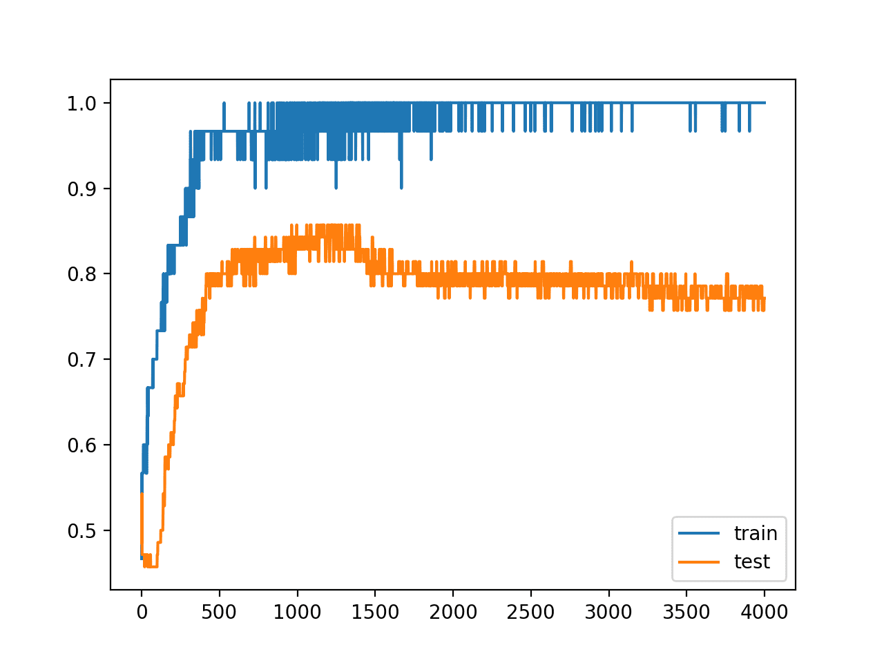
Line Plot of Train and Test Accuracy With Input Layer Noise
MLP With Hidden Layer Noise
An alternative approach to adding noise to the input values is to add noise between the hidden layers.
This can be done by adding noise to the linear output of the layer (weighted sum) before the activation function is applied, in this case a rectified linear activation function. We can also use a larger standard deviation for the noise as the model is less sensitive to noise at this level given the presumably larger weights from being overfit. We will use a standard deviation of 0.1, again, chosen arbitrarily.
|
1 2 3 4 5 6 7 |
# define model model = Sequential() model.add(Dense(500, input_dim=2)) model.add(GaussianNoise(0.1)) model.add(Activation('relu')) model.add(Dense(1, activation='sigmoid')) model.compile(loss='binary_crossentropy', optimizer='adam', metrics=['accuracy']) |
The complete example with Gaussian noise between the hidden layers is listed below.
|
1 2 3 4 5 6 7 8 9 10 11 12 13 14 15 16 17 18 19 20 21 22 23 24 25 26 27 28 29 30 31 |
# mlp overfit on the two circles dataset with hidden layer noise from sklearn.datasets import make_circles from keras.models import Sequential from keras.layers import Dense from keras.layers import Activation from keras.layers import GaussianNoise from matplotlib import pyplot # generate 2d classification dataset X, y = make_circles(n_samples=100, noise=0.1, random_state=1) # split into train and test n_train = 30 trainX, testX = X[:n_train, :], X[n_train:, :] trainy, testy = y[:n_train], y[n_train:] # define model model = Sequential() model.add(Dense(500, input_dim=2)) model.add(GaussianNoise(0.1)) model.add(Activation('relu')) model.add(Dense(1, activation='sigmoid')) model.compile(loss='binary_crossentropy', optimizer='adam', metrics=['accuracy']) # fit model history = model.fit(trainX, trainy, validation_data=(testX, testy), epochs=4000, verbose=0) # evaluate the model _, train_acc = model.evaluate(trainX, trainy, verbose=0) _, test_acc = model.evaluate(testX, testy, verbose=0) print('Train: %.3f, Test: %.3f' % (train_acc, test_acc)) # plot history pyplot.plot(history.history['accuracy'], label='train') pyplot.plot(history.history['val_accuracy'], label='test') pyplot.legend() pyplot.show() |
Running the example reports the model performance on the train and test datasets.
Note: Your results may vary given the stochastic nature of the algorithm or evaluation procedure, or differences in numerical precision. Consider running the example a few times and compare the average outcome.
In this case, we can see a marked increase in the performance of the model on the hold out test set.
|
1 |
# Train: 0.967, Test: 0.814 |
We can also see from the line plot of accuracy over training epochs that the model no longer appears to show the properties of being overfit.
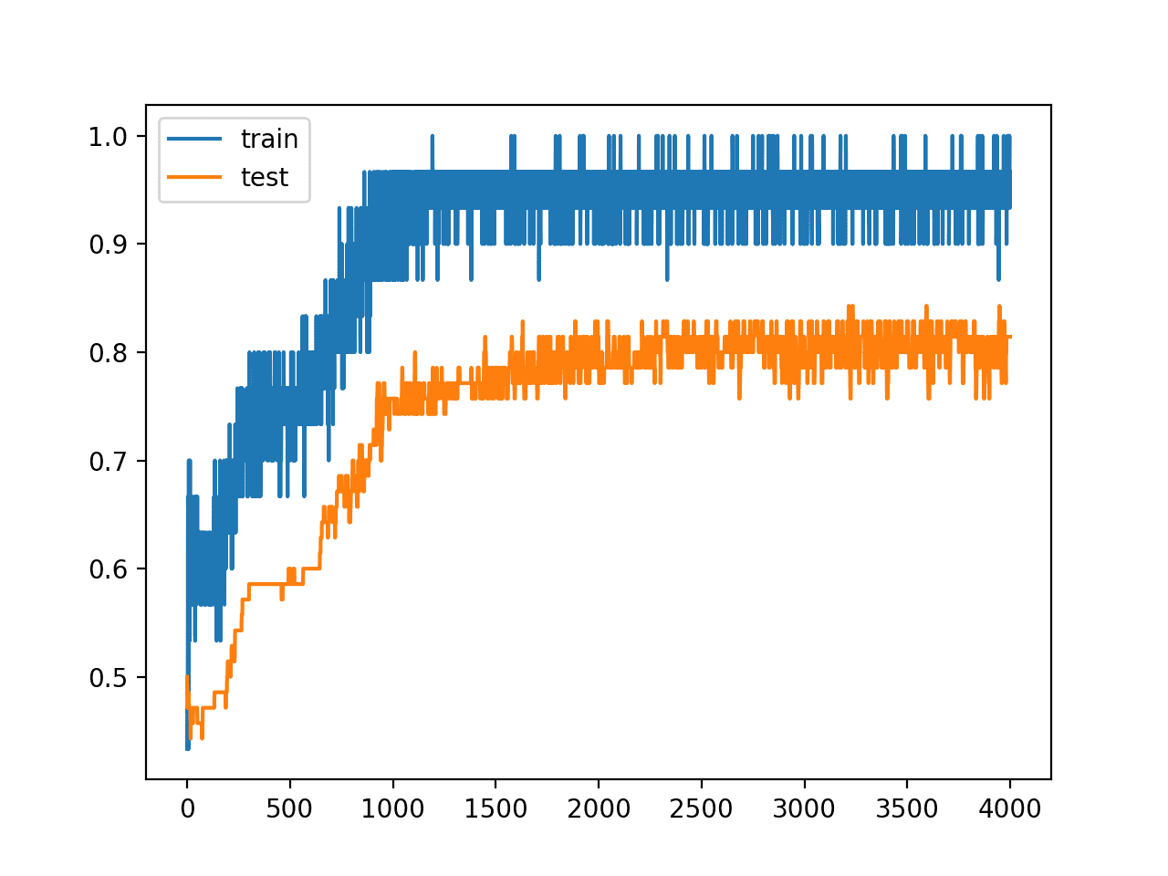
Line Plot of Train and Test Accuracy With Hidden Layer Noise
We can also experiment and add the noise after the outputs of the first hidden layer pass through the activation function.
|
1 2 3 4 5 6 |
# define model model = Sequential() model.add(Dense(500, input_dim=2, activation='relu')) model.add(GaussianNoise(0.1)) model.add(Dense(1, activation='sigmoid')) model.compile(loss='binary_crossentropy', optimizer='adam', metrics=['accuracy']) |
The complete example is listed below.
|
1 2 3 4 5 6 7 8 9 10 11 12 13 14 15 16 17 18 19 20 21 22 23 24 25 26 27 28 29 |
# mlp overfit on the two circles dataset with hidden layer noise (alternate) from sklearn.datasets import make_circles from keras.models import Sequential from keras.layers import Dense from keras.layers import GaussianNoise from matplotlib import pyplot # generate 2d classification dataset X, y = make_circles(n_samples=100, noise=0.1, random_state=1) # split into train and test n_train = 30 trainX, testX = X[:n_train, :], X[n_train:, :] trainy, testy = y[:n_train], y[n_train:] # define model model = Sequential() model.add(Dense(500, input_dim=2, activation='relu')) model.add(GaussianNoise(0.1)) model.add(Dense(1, activation='sigmoid')) model.compile(loss='binary_crossentropy', optimizer='adam', metrics=['accuracy']) # fit model history = model.fit(trainX, trainy, validation_data=(testX, testy), epochs=4000, verbose=0) # evaluate the model _, train_acc = model.evaluate(trainX, trainy, verbose=0) _, test_acc = model.evaluate(testX, testy, verbose=0) print('Train: %.3f, Test: %.3f' % (train_acc, test_acc)) # plot history pyplot.plot(history.history['accuracy'], label='train') pyplot.plot(history.history['val_accuracy'], label='test') pyplot.legend() pyplot.show() |
Running the example reports the model performance on the train and test datasets.
Note: Your results may vary given the stochastic nature of the algorithm or evaluation procedure, or differences in numerical precision. Consider running the example a few times and compare the average outcome.
Surprisingly, we see little difference in the performance of the model.
|
1 |
Train: 0.967, Test: 0.814 |
Again, we can see from the line plot of accuracy over training epochs that the model no longer shows sign of overfitting.
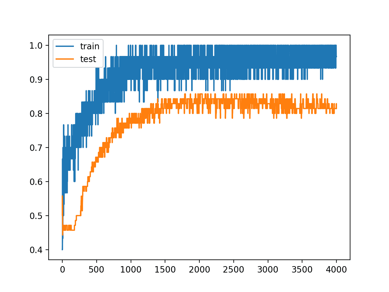
Line Plot of Train and Test Accuracy With Hidden Layer Noise (alternate)
Extensions
This section lists some ideas for extending the tutorial that you may wish to explore.
- Repeated Evaluation. Update the example to use repeated evaluation of the model with and without noise and report performance as the mean and standard deviation over repeats.
- Grid Search Standard Deviation. Develop a grid search in order to discover the amount of noise that reliably results in the best performing model.
- Input and Hidden Noise. Update the example to introduce noise at both the input and hidden layers of the model.
If you explore any of these extensions, I’d love to know.
Further Reading
This section provides more resources on the topic if you are looking to go deeper.
- Keras Regularizers API
- Keras Core Layers API
- Keras Convolutional Layers API
- Keras Recurrent Layers API
- Keras Noise API
- sklearn.datasets.make_circles API
Summary
In this tutorial, you discovered how to add noise to deep learning models in Keras in order to reduce overfitting and improve model generalization.
Specifically, you learned:
- Noise can be added to a neural network model via the GaussianNoise layer.
- The GaussianNoise can be used to add noise to input values or between hidden layers.
- How to add a GaussianNoise layer in order to reduce overfitting in a Multilayer Perceptron model for classification.
Do you have any questions?
Ask your questions in the comments below and I will do my best to answer.


Thanks Jason, nicely explained. Really enjoyed it.
Thanks.
Thanks, but I think we only have Gaussian noise layer. if I want to apply some attacks like cropping, do we have any layer in keras for this? do you have any suggestion for this? I look forward to hearing from you.
Good question, generally no, you can use a custom data generator and perform random crops to images before they are fed into the model.
Hi Jason, what do you think about backward pass when you add noise to either weights or activations? For example, when adding noise to activations (which serve as layer inputs), to calculate weight gradients for that layer, you multiply incoming gradient by these activations. Would you use the original activations, or the distorted ones? Or when backpropagating errors we multiply them by transposed weight matrices in each layer, again, would you use the original weights or distorted ones?
Hmmm.
I have not see it often, except with models like GANs and stochastic label smoothing – required only because training GANs is so unstable.
If you have an idea, try it. It has never been easier with such amazing tools!
It actually does not seem easy to me. For example, say we want to add noise to activations (inputs to second layer), and then update weights of that second layer. Standard autodiff in either TF or Pytorch would pass upstream gradients right through the noise addition op, to be multiplied by the original second layer inputs. But how can I change this so that they get multiplied by the distorted inputs? I don’t think the distorted inputs are being preserved for the backward pass.
In this case, I think the tools actually make it harder to experiment.
Or, if it is the distorted inputs that are being preserved by autodiff, then how do I skip them and pass the gradients to the original ones?
The model does not see distorted inputs, it sees inputs/outputs/activations. It just so happens that you’ve distorted them with noise. Updates happen per normal.
Perhaps I don’t follow the nuance of what you’re trying to implement.
Hello Jason,
I was wondering, if a layer of noise is added to the model architecture, would it then apply that noise to every test input as well? How would you go about training a model with noise, and then training with clean inputs?
It depends. Input or output noise is usually turned off, sometimes it is left on a test time. Noise within the model is sometime left on. Perhaps eval with/without at test time and compare.
If you wanted, you could reformulate the final model without the noise layer.
Hi Jason,
Great article, I have a question regarding the use of Gaussian Noise over some input that has been previously padded (with 0’s for example). Do you think the loss in the training could get worse in this case? An example could be padding different length inputs like speech spectrograms in order for them to have the same shape.
Hmm, good question.
Yes, noise over padding sounds like a bad idea.
There are many ways to get noise into the system, get creative and test a suite of approaches.
Hi! Is there also a simple way to tinker/augment the contrast? Something like model.add(Contrast(0.1))?
For images, yes, you can use data augmentation:
https://machinelearningmastery.com/how-to-configure-image-data-augmentation-when-training-deep-learning-neural-networks/
I want to to add some noise to the neural network I am using for the classification of jpg images. So, the input for my neural network are arrays of the pixels, that I have already normalized to be in the range 0 to 1. I wanted to do as in your suggestion:
…
model.add(MaxPooling2D())
model.add(GaussianNoise(x))
…
But I am concerned that the GaussianNoise might make my data go outside the range 0 to 1 and spoil the training. Is this a valid concern or am I safe? Does it depend on the value x to be used in model.add(GaussianNoise(x)) and what x value would you use? Thanks
It should be fine, perhaps test it and evaluate the effects?
Alternately, you could create your own custom layer to achieve exactly what you want.
Hi Jason,
Thank you for this tutorial!.
I have been playing with this tutorial adding other options to the script in order to experiment with them in a kind of “grid search”. Here it is my report.
– I define my models with keras model class API instead of Sequential: But I do not expect any impact on results (!).
– I set up the model (as you) but also I used other “high level” model constructor such as ‘KerasClassifier’ and ‘cross_val_score’ (for Kfold statical analysis) from Sklearn library, taken from other tutorial from you. In general the ‘cross_val_score’ got less average accuracy (69% mean accuracy) in front of 85.7% accuracy for model on test input. I understand it.
But curiously I got in general better results when I use the KerasClassiffier (e.g. 84.3%).
And I do not understand why I got better results on kerasclassifier than in my “manual” API class model if I am using the same “validation_split” in both cases (70% for test 30% for input training).
– I got the same validation training results of some kind of “sinusoidal loss curve” (going down and up but with the long trend going up even when I re-train up to 8000 epochs ). And same effect on validation accuracy but little downing trend). All these cases applying with not adding gaussian noise.
– I observed that X input data coming from “make_circles of sklearn are between -1.06… and + 1.06 …so I decided to normalize or standardize the input data (with MinMaxScaler and StandardScaler from sklearn and from yours tutorials. In general I got a little better performance on ‘cross-val-score. ( It is increased up t0 to 72% mean accuracy) , but better for my kerasClassifier (up to 88.6% accuracy) but a little worst for my “manual model” around 77% Accuracy on test.
-the bing results sensitivity is when I decided to permute the 70% test and 30% training input for 30% test and 70% training (more natural exploitation of data). In this case I got 83% mean accuracy on cross_val_score with a sigma of 10.7% and 96.7 accuracy from Kerasclassifier and 90% accuracy for my manual model. it is clear the reason in this scenario.
-Also I performed Dropout layers and weight constraint regularization (taken from your tutorials) but the results are not so much different.
– I apply of course the Gaussian noise layer (after input or before output layer) , And clearly I obtain the right trend in terms of validation loss training curve (disappearing the loss increase in validation during training epochs increase), but I do get similar accuracy for my manual model and a little better for the scross-val-score constructor. I Observed that are very sensitivity to the sigma (estandard deviation figure) apply to the gaussian noise layer.
– Even I apply everything for regularization altogether in a kind of ‘totum revolutum’ (dropout layer + gaussian noise + weight constraint regularization ) plus input data scaler … I get accuracy around 50% (not learning at all) so it is clear that I need more control for every of these tools…:-)
– As a summary I do not get so much impact on accuracy results when apply gaussian noise layer (but of course better behavior on loss and accuracy training curves) when using gaussian noise layer (even when using both of them layer after input and before output at the same time)…probably because sigma noise (standard deviation) has to be better fit …
thank you for your tutorial Jason
Wonderful experimentation, thanks for sharing.
This would be valuable stuff if you write it up and shared it – valuable as in it shows how systematic and curious one must be to really dive into these techniques.
Adding noise was really popular in the 90s, less so now that we have dropout. Yet, I see it popup in big modern gan models, so it’s still around and useful.
Hey Jason, great article.
How would you add input noise to a pre-trained model such as:
from tensorflow.keras.applications.resnet50 import ResNet50
I just want to do input noise, but I’m struggling on how to insert it.
Add a noise layer as the first layer of the mode – e.g. with the functional api.
Perhaps I don’t understand the problem?
Hi Jason
Thanks for your great explanations
Do you have any suggestion for any document that studies the robustness of LSTM to training noise
Thanks
Not off hand, perhaps run a sensitivity analysis on your dataset?
I have added noise layer to my model and i have got the same results as before adding that noisy layer? Does that mean my model good or overfitting ?
Hi Alex…The following resource may be of interest to you:
https://machinelearningmastery.com/overfitting-machine-learning-models/