Optimization is a big part of machine learning. It is the core of most popular methods, from least squares regression to artificial neural networks.
In this post you will discover recipes for 5 optimization algorithms in R.
These methods might be useful in the core of your own implementation of a machine learning algorithm. You may want to implement your own algorithm tuning scheme to optimize the parameters of a model for some cost function.
A good example may be the case where you want to optimize the hyper-parameters of a blend of predictions from an ensemble of multiple child models.
Kick-start your project with my new book Machine Learning Mastery With R, including step-by-step tutorials and the R source code files for all examples.
Let’s get started.
Golden Section Search
Golden Section Search is a Line Search method for Global Optimization in one-dimension. It is a Direct Search (Pattern Search) method as it samples the function to approximate a derivative rather than computing it directly.
The Golden Section Search is related to pattern searches of discrete ordered lists such as the Binary Search and the Fibonacci Search. It is related to other Line Search algorithms such as Brent’s Method and more generally to other direct search optimization methods such as the Nelder-Mead Method.
The information processing objective of the method is to locate the extremum of a function. It does this by directly sampling the function using a pattern of three points. The points form the brackets on the search: the first and the last points are the current bounds of the search, and the third point partitions the intervening space. The partitioning point is selected so that the ratio between the larger partition and the whole interval is the same as the ratio of the larger partition to the small partition, known as the golden ratio (phi). The partitions are compared based on their function evaluation and the better performing section is selected as the new bounds on the search. The process recurses until the desired level of precision (bracketing of the optimum) is obtained or the search stalls.
The following example provides a code listing Golden Section Search method in R solving a one-dimensional nonlinear unconstrained optimization function.
Golden Section Search in R
R
1
2
3
4
5
6
7
8
9
10
11
12
13
14
15
16
17
18
19
20
21
22
23
24
# define a 1D basin function, optima at f(0)=0
basin<-function(x){
x[1]^2
}
# locate the minimum of the function using a Golden Section Line Search
result<-optimize(
basin,# the function to be minimized
c(-5,5),# the bounds on the function parameter
maximum=FALSE,# we are concerned with the function minima
Assumes that the function is convex and unimodal specifically, that the function has a single optimum and that it lies between the bracketing points.
Intended to find the extrema one-dimensional continuous functions.
It was shown to be more efficient than an equal-sized partition line search.
The termination criteria is a specification on the minimum distance between the brackets on the optimum.
It can quickly locate the bracketed area of the optimum but is less efficient at locating the specific optimum.
Once a solution of desired precision is located, it can be provided as the basis to a second search algorithm that has a faster rate of convergence.
Need more Help with R for Machine Learning?
Take my free 14-day email course and discover how to use R on your project (with sample code).
Click to sign-up and also get a free PDF Ebook version of the course.
Nelder Mead
The Nelder-Mead Method is an optimization algorithm for multidimensional nonlinear unconstrained functions.
It is a Direct Search Method in that it does not use a function gradient during the procedure. It is a Pattern Search in that it uses a geometric pattern to explore the problem space.
It is related to other Direct Search optimization methods such as Hooke and Jeeves’ Pattern Search that also uses a geometric pattern to optimize an objective function.
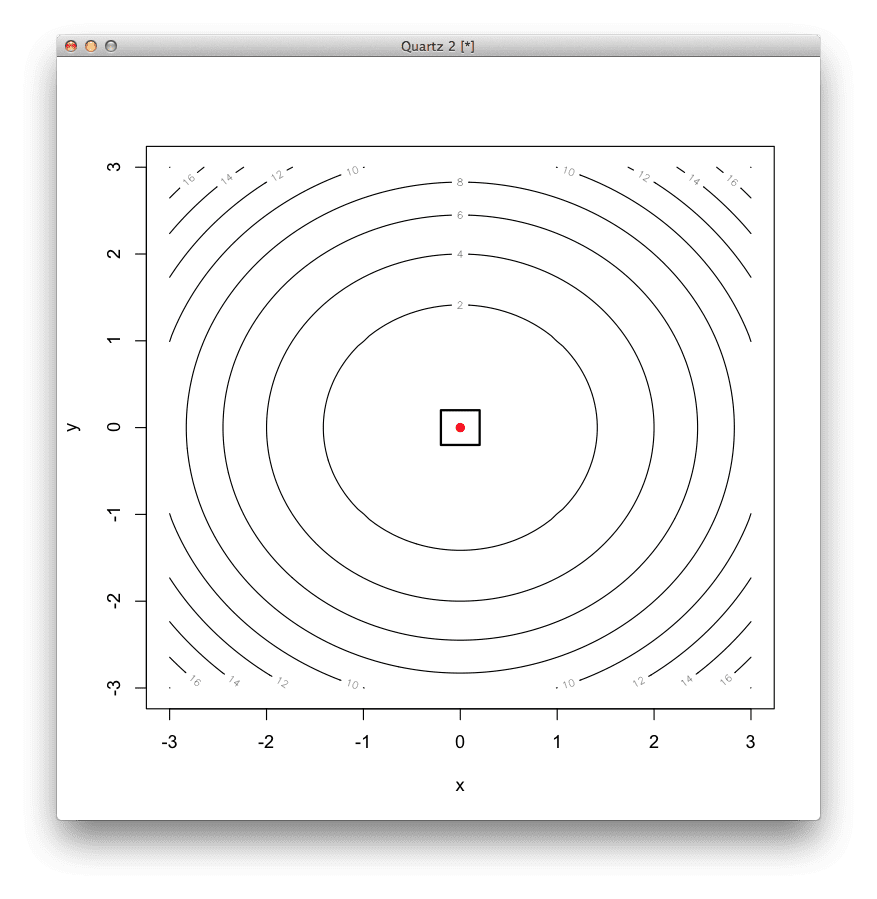
The information processing objective of the Nelder-Mead Method is to locate the extremum of a function. This is achieved by overlaying a simplex (geometrical pattern) in the domain and iteratively increasing and/or reducing its size until an optimal value is found. The simplex is defined always with n+1 vertices, where n is the number of dimensions of the search space (i.e. a triangle for a 2D problem).
The process involves identifying the worst performing point of the complex and replacing it with a point reflected through the centroid (center point) of the remaining points. The simplex can be deformed (adapt itself to the topology of the search space) by expanding away from the worst point, contract along one dimension away from the worst point, or contract on all dimensions towards the best point.
The following example provides a code listing of the Nelder-Mead method in R solving a two-dimensional nonlinear optimization function.
Nelder-Mead Method in R
R
1
2
3
4
5
6
7
8
9
10
11
12
13
14
15
16
17
18
19
20
21
22
23
24
25
26
27
28
29
30
31
32
33
34
35
# definition of the 2D Rosenbrock function, optima is at (1,1)
rosenbrock<-function(v){
(1-v[1])^2+100*(v[2]-v[1]*v[1])^2
}
# locate the minimum of the function using the Nelder-Mead method
result<-optim(
c(runif(1,-3,3),runif(1,-3,3)),# start at a random position
It can be used with multi-dimensional functions (one or more parameters) and with non-linear response surfaces.
It does not use a function derivative meaning that it can be used on non-differentiable functions, discontinuous functions, non-smooth functions, and noisy functions.
As a direct search method it is consider inefficient and slow relative to modern derivative-based methods.
It is dependent on the starting position and can be caught by local optimum in multimodal functions.
The stopping criteria can be a minimum change in the best position.
The nature of the simplex structure can mean it can get stuck in non-optimal areas of the search space, this is more likely if the size of the initial simplex is too large.
When the method does work (is appropriate for the function being optimized) it has been shown to be fast and robust.
Gradient Descent
Gradient Descent is a first-order derivative optimization method for unconstrained nonlinear function optimization. It is called Gradient Descent because it was envisioned for function minimization. When applied to function maximization it may be referred to as Gradient Ascent.
Steepest Descent Search is an extension that performs a Line Search on the line of the gradient to the locate the optimum neighboring point (optimum step or steepest step). Batch Gradient Descent is an extension where the cost function and its derivative are computed as the summed error on a collection of training examples. Stochastic Gradient Descent (or Online Gradient Descent) is like Batch Gradient Descent except that the cost function and derivative are computed for each training example.
The information processing objective of the method is to locate the extremum of a function. This is achieved by first selecting a starting point in the search space. For a given point in the search space, the derivative of the cost function is calculated and a new point is selected down the gradient of the functions derivative at a distance of alpha (the step size parameter) from the current point.
The example provides a code listing Gradient Descent algorithm in R solving a two-dimensional nonlinear optimization function.
The method is limited to finding the local optimum, which if the function is convex, is also the global optimum.
It is considered inefficient and slow (linear) to converge relative to modern methods. Convergence can be slow if the gradient at the optimum flattens out (gradient goes to 0 slowly). Convergence can also be slow if the Hessian is poorly conditioned (gradient changes rapidly in some directions and slower in others).
The step size (alpha) may be constant, may adapt with the search, and may be maintained holistically or for each dimension.
The method is sensitive to initial conditions, and as such, it can be common to repeat the search process a number of times with randomly selected initial positions.
If the step size parameter (alpha) is too small, the search will generally take a large number of iterations to converge, if the parameter is too large can overshoot the function’s optimum.
Compared to non-iterative function optimization methods, gradient descent has some relative efficiencies when it comes to scaling with the number of features (dimensions).
Conjugate Gradient
Conjugate Gradient Method is a first-order derivative optimization method for multidimensional nonlinear unconstrained functions. It is related to other first-order derivative optimization algorithms such as Gradient Descent and Steepest Descent.
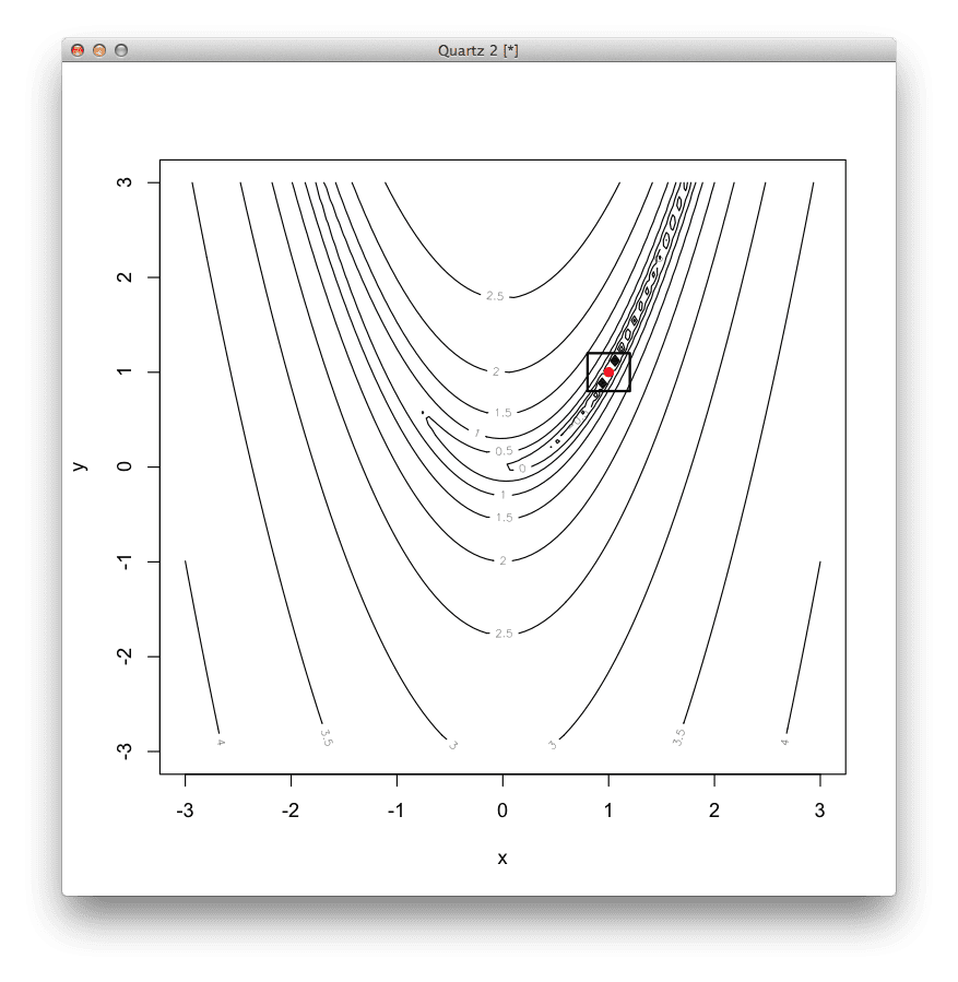
The information processing objective of the technique is to locate the extremum of a function. From a starting position, the method first computes the gradient to locate the direction of steepest descent, then performs a line search to locate the optimum step size (alpha). The method then repeats the process of computing the steepest direction, computes direction of the search, and performing a line search to locate the optimum step size. A parameter beta defines the direction update rule based on the gradient and can be computed using one of a number of methods.
The difference between Conjugate Gradient and Steepest Descent is that it uses conjugate directions rather than local gradients to move downhill towards the function minimum, which can be very efficient.
The example provides a code listing of the Conjugate Gradient method in R solving a two-dimensional nonlinear optimization function.
Conjugate Gradient in R
R
1
2
3
4
5
6
7
8
9
10
11
12
13
14
15
16
17
18
19
20
21
22
23
24
25
26
27
28
29
30
31
32
33
34
35
36
# definition of the 2D Rosenbrock function, optima is at (1,1)
rosenbrock<-function(v){
(1-v[1])^2+100*(v[2]-v[1]*v[1])^2
}
# definition of the gradient of the 2D Rosenbrock function
derivative<-function(v){
c(-400*v[1]*(v[2]-v[1]*v[1])-2*(1-v[1]),
200*(v[2]-v[1]*v[1]))
}
# locate the minimum of the function using the Conjugate Gradient method
result<-optim(
c(runif(1,-3,3),runif(1,-3,3)),# start at a random position
rosenbrock,# the function to minimize
derivative,# no function gradient
method="CG",# use the Conjugate Gradient method
control=c(# configure Conjugate Gradient
maxit=100,# maximum iterations of 100
reltol=1e-8,# response tolerance over-one step
type=2))# use the Polak-Ribiere update method
# summarize results
print(result$par)# the coordinate of the minimum
print(result$value)# the function response of the minimum
print(result$counts)# the number of function calls performed
It is more efficient than Steepest Descent, for example it may take a straight line path down narrow valley’s, whereas Steepest Descent would have to zig-zag (pinball) down the valley.
Devolves into Steepest Descent if the conjugate direction is reset each iteration.
It is almost as fast as second-order gradient methods, requiring just n iterations to locate an optimum for suitable functions (where n is the number of parameters).
It does not maintain a Hessian matrix (like BFGS) and therefore may be suitable for larger problems with many variables.
The method is most efficient (works the best) with quadratic or quadratic-like functions, or where the function is approximately quadratic near the optimum.
The method is sensitive to its starting position on non-convex problems.
The learning rate (step size alpha) does not have to be specified as a line search is used to locate the optimum value as needed.
Common methods for computing the direction update rule (beta) are the Hestenes-Stiefel, Fletcher-Reeves, Polak-Ribiere, and Beale-Sorenson methods. The Polak-Ribiere method generally works better in practice for non-quadratic functions.
It is dependent on the accuracy of the line search, errors introduced both from this and the less-than quadratic nature of the response surface will result in more frequent updates to the direction and a less efficient search.
To avoid the search degenerating, consider restarting the search process after n iterations, where n is the number of function parameters.
BFGS
BFGS is an optimization method for multidimensional nonlinear unconstrained functions.
BFGS belongs to the family of quasi-Newton (Variable Metric) optimization methods that make use of both first-derivative (gradient) and second-derivative (Hessian matrix) based information of the function being optimized. More specifically, it is a quasi-Newton method which means that it approximates the second-order derivative rather than compute it directly. It is related to other quasi-Newton methods such as the DFP Method, Broyden’s method and the SR1 Method.
Two popular extension of BFGS is L-BFGS (Limited Memory BFGS) which has lower memory resource requirements and L-BFGS-B (Limited Memory Boxed BFGS) which extends L-BFGS and imposes box constraints on the method.
The information processing objective of the BFGS Method is to locate the extremum of a function.
This is achieved by iteratively building up a good approximation of the inverse Hessian matrix. Given an initial starting position, it prepares an approximation of the Hessian matrix (square matrix of second-order partial derivatives). It then repeats the process of computing the search direction using the approximated Hessian, computes an optimum step size using a Line Search then, updates the position, and updates the approximation of the Hessian. The method for updating the Hessian each iteration is called the BFGS rule which insures the updated matrix is positive definite.
The example provides a code listing of the BFGS method in R solving a two-dimensional nonlinear optimization function.
BFGS in R
R
1
2
3
4
5
6
7
8
9
10
11
12
13
14
15
16
17
18
19
20
21
22
23
24
25
26
27
28
29
30
31
32
33
34
# definition of the 2D Rosenbrock function, optima is at (1,1)
rosenbrock<-function(v){
(1-v[1])^2+100*(v[2]-v[1]*v[1])^2
}
# definition of the gradient of the 2D Rosenbrock function
It requires a function where the the functions gradient (first partial derivative) can be computed at arbitrary points.
It does not require second-order derivatives as it approximates the Hessian matrix, making it less computationally expensive compared to Newton’s method.
It requires a relatively large memory footprint, as it maintains an n*n Hessian matrix, where n is the number of variables. This is a limitation on the methods scalability.
The rate of convergence is super-linear and the computational cost of each iteration is O(n^2).
The L-BFGS extension to BFGS is intended for functions with very large numbers of parameters (>1000).
The stopping condition is typically a minimum change is response or a minimum gradient.
BFGS is somewhat robust and self correcting in terms of the search direction and as such it does not require the use of exact line searches when determining the step size.
Summary
Optimization is an important concept to understand and apply carefully in applied machine learning.
In this post you discovered 5 convex optimization algorithms with recipes in R that are ready to copy and paste into your own problem.
You also learned some background for each method and general heuristics for operating each algorithm.
Did I miss your favorite convex optimization algorithm? Leave a comment and let me know.
I currently carry on this LASSO related project in R. However, out of specific need of research , I have to change the penalty function to another smooth function. The problem is I was totally spoiled by all the well-established packages in R to solve all kinds of PLS problems. I have used “glmnet” to solve LASSO, ridge and elastic-net, used “ncvreg” to solve SCAD. But I don’t know which general optimization package I should use to make a refinement on the restriction function for my own purpose. Could you please shed some light on my dilemma? I will greatly appreciate your help and suggestions.
I am a retired scientist, a Ph.D in Mathematics, specialized in optimization techniques and an IT fellow.
Your article ‘Convex Optimization in R’ has aroused my interest in learning Machine Learning. Could you help me by sending your literature and collection of literature on Machine Learning. This associate may last longer and it may give many a tools and techniques to data analytics and optimization communities !!!!
Wishing a great success in your all ventures, I am
Dr. R. K. VERMA
I appreciate your examples on Convex Optimization in R.
My suggestion: You release a series on ‘Optimization Methods in R’ ranging from linear programming thru to non-linear programming. OR/MS community in academia and industry will highly appreciate such a series, believe me.


")


I currently carry on this LASSO related project in R. However, out of specific need of research , I have to change the penalty function to another smooth function. The problem is I was totally spoiled by all the well-established packages in R to solve all kinds of PLS problems. I have used “glmnet” to solve LASSO, ridge and elastic-net, used “ncvreg” to solve SCAD. But I don’t know which general optimization package I should use to make a refinement on the restriction function for my own purpose. Could you please shed some light on my dilemma? I will greatly appreciate your help and suggestions.
Dear Jason,
I am a retired scientist, a Ph.D in Mathematics, specialized in optimization techniques and an IT fellow.
Your article ‘Convex Optimization in R’ has aroused my interest in learning Machine Learning. Could you help me by sending your literature and collection of literature on Machine Learning. This associate may last longer and it may give many a tools and techniques to data analytics and optimization communities !!!!
Wishing a great success in your all ventures, I am
Dr. R. K. VERMA
Dear Jason,
I appreciate your examples on Convex Optimization in R.
My suggestion: You release a series on ‘Optimization Methods in R’ ranging from linear programming thru to non-linear programming. OR/MS community in academia and industry will highly appreciate such a series, believe me.
Wishing a great success once more, I am
Dr. R. K. Verma
Do you have any code for Gradient Descent Method for constrained inequality functions? If so, please share.That would be a great help.
I don’t believe so.
Hi Thanks for the article, that’s very useful.
I get an error on contour command:
Error in contour.default(x, y, matrix(log10(z), length(x)), xlab = “x”, : no proper ‘z’ matrix specified
May I ask what is wrong?
when I print the matrix, it is what I get:
[,1]
[1,] Numeric,10000
[2,] Numeric,10000
for 100 times.
May I ask what is wrong and how can I fix it? Thanks!
Perhaps the API has changed since the code was written?