Bootstrap aggregation, or bagging, is an ensemble where each model is trained on a different sample of the training dataset.
The idea of bagging can be generalized to other techniques for changing the training dataset and fitting the same model on each changed version of the data. One approach is to use data transforms that change the scale and probability distribution of input variables as the basis for the training of contributing members to a bagging-like ensemble. We can refer to this as data transform bagging or a data transform ensemble.
In this tutorial, you will discover how to develop a data transform ensemble.
After completing this tutorial, you will know:
- Data transforms can be used as the basis for a bagging-type ensemble where the same model is trained on different views of a training dataset.
- How to develop a data transform ensemble for classification and confirm the ensemble performs better than any contributing member.
- How to develop and evaluate a data transform ensemble for regression predictive modeling.
Kick-start your project with my new book Ensemble Learning Algorithms With Python, including step-by-step tutorials and the Python source code files for all examples.
Let’s get started.

Develop a Bagging Ensemble with Different Data Transformations
Photo by Maciej Kraus, some rights reserved.
Tutorial Overview
This tutorial is divided into three parts; they are:
- Data Transform Bagging
- Data Transform Ensemble for Classification
- Data Transform Ensemble for Regression
Data Transform Bagging
Bootstrap aggregation, or bagging for short, is an ensemble learning technique based on the idea of fitting the same model type on multiple different samples of the same training dataset.
The hope is that small differences in the training dataset used to fit each model will result in small differences in the capabilities of models. For ensemble learning, this is referred to as diversity of ensemble members and is intended to de-correlate the predictions (or prediction errors) made by each contributing member.
Although it was designed to be used with decision trees and each data sample is made using the bootstrap method (selection with rel-selection), the approach has spawned a whole subfield of study with hundreds of variations on the approach.
We can construct our own bagging ensembles by changing the dataset used to train each contributing member in new and unique ways.
One approach would be to apply a different data preparation transform to the dataset for each contributing ensemble member.
This is based on the premise that we cannot know the representational form for a training dataset that exposes the unknown underlying structure to the dataset to the learning algorithms. This motivates the need to evaluate models with a suite of different data transforms, such as changing the scale and probability distribution, in order to discover what works.
This approach can be used where a suite of different transforms of the same training dataset is created, a model trained on each, and the predictions combined using simple statistics such as averaging.
For lack of a better name, we will refer to this as “Data Transform Bagging” or a “Data Transform Ensemble.”
There are many transforms that we can use, but perhaps a good starting point would be a selection that changes the scale and probability distribution, such as:
- Normalization (fixed range)
- Standardization (zero mean)
- Robust Standardization (robust to outliers)
- Power Transform (remove skew)
- Quantile Transform (change distribution)
- Discretization (k-bins)
The approach is likely to be more effective when used with a base model that trains different or very different models based on the effects of the data transform.
Changing the scale of the distribution may only be appropriate with models that are sensitive to changes in the scale of input variables, such as those that calculate a weighted sum, such as logistic regression and neural networks, and those that use distance measures, such as k-nearest neighbors and support vector machines.
Changes to the probability distribution for input variables would likely impact most machine learning models.
Now that we are familiar with the approach, let’s explore how we can develop a data transform ensemble for classification problems.
Want to Get Started With Ensemble Learning?
Take my free 7-day email crash course now (with sample code).
Click to sign-up and also get a free PDF Ebook version of the course.
Data Transform Ensemble for Classification
We can develop a data transform approach to bagging for classification using the scikit-learn library.
The library provides a suite of standard transforms that we can use directly. Each ensemble member can be defined as a Pipeline, with the transform followed by the predictive model, in order to avoid any data leakage and, in turn, produce optimistic results. Finally, a voting ensemble can be used to combine the predictions from each pipeline.
First, we can define a synthetic binary classification dataset as the basis for exploring this type of ensemble.
The example below creates a dataset with 1,000 examples each comprising 20 input features, where 15 of them contain information for predicting the target.
|
1 2 3 4 5 6 |
# synthetic classification dataset from sklearn.datasets import make_classification # define dataset X, y = make_classification(n_samples=1000, n_features=20, n_informative=15, n_redundant=5, random_state=1) # summarize the dataset print(X.shape, y.shape) |
Running the example will create the dataset and summarizes the shape of the data arrays, confirming our expectations.
|
1 |
(1000, 20) (1000,) |
Next, we establish a baseline on the problem using the predictive model we intend to use in our ensemble. It is standard practice to use a decision tree in bagging ensembles, so in this case, we will use the DecisionTreeClassifier with default hyperparameters.
We will evaluate the model using standard practices, in this case, repeated stratified k-fold cross-validation with three repeats and 10 folds. The performance will be reported using the mean of the classification accuracy across all folds and repeats.
The complete example of evaluating a decision tree on the synthetic classification dataset is listed below.
|
1 2 3 4 5 6 7 8 9 10 11 12 13 14 15 16 17 |
# evaluate decision tree on synthetic classification dataset from numpy import mean from numpy import std from sklearn.datasets import make_classification from sklearn.model_selection import cross_val_score from sklearn.model_selection import RepeatedStratifiedKFold from sklearn.tree import DecisionTreeClassifier # define dataset X, y = make_classification(n_samples=1000, n_features=20, n_informative=15, n_redundant=5, random_state=1) # define the model model = DecisionTreeClassifier() # define the evaluation procedure cv = RepeatedStratifiedKFold(n_splits=10, n_repeats=3, random_state=1) # evaluate the model n_scores = cross_val_score(model, X, y, scoring='accuracy', cv=cv, n_jobs=-1) # report performance print('Mean Accuracy: %.3f (%.3f)' % (mean(n_scores), std(n_scores))) |
Running the example reports the mean classification accuracy of the decision tree on the synthetic classification dataset.
Note: Your results may vary given the stochastic nature of the algorithm or evaluation procedure, or differences in numerical precision. Consider running the example a few times and compare the average outcome.
In this case, we can see that the model achieved a classification accuracy of about 82.3 percent.
This score provides a baseline in performance from which we expect a data transform ensemble to improve upon.
|
1 |
Mean Accuracy: 0.823 (0.039) |
Next, we can develop an ensemble of decision trees, each fit on a different transform of the input data.
First, we can define each ensemble member as a modeling pipeline. The first step will be the data transform and the second will be a decision tree classifier.
For example, the pipeline for a normalization transform with the MinMaxScaler class would look as follows:
|
1 2 3 |
... # normalization norm = Pipeline([('s', MinMaxScaler()), ('m', DecisionTreeClassifier())]) |
We can repeat this for each transform or transform configuration that we want to use and add all of the model pipelines to a list.
The VotingClassifier class can be used to combine the predictions from all of the models. This class takes an “estimators” argument that is a list of tuples where each tuple has a name and the model or modeling pipeline. For example:
|
1 2 3 4 5 6 7 |
... # normalization norm = Pipeline([('s', MinMaxScaler()), ('m', DecisionTreeClassifier())]) models.append(('norm', norm)) ... # define the voting ensemble ensemble = VotingClassifier(estimators=models, voting='hard') |
To make the code easier to read, we can define a function get_ensemble() to create the members and data transform ensemble itself.
|
1 2 3 4 5 6 7 8 9 10 11 12 13 14 15 16 17 18 19 20 21 22 23 24 25 |
# get a voting ensemble of models def get_ensemble(): # define the base models models = list() # normalization norm = Pipeline([('s', MinMaxScaler()), ('m', DecisionTreeClassifier())]) models.append(('norm', norm)) # standardization std = Pipeline([('s', StandardScaler()), ('m', DecisionTreeClassifier())]) models.append(('std', std)) # robust robust = Pipeline([('s', RobustScaler()), ('m', DecisionTreeClassifier())]) models.append(('robust', robust)) # power power = Pipeline([('s', PowerTransformer()), ('m', DecisionTreeClassifier())]) models.append(('power', power)) # quantile quant = Pipeline([('s', QuantileTransformer(n_quantiles=100, output_distribution='normal')), ('m', DecisionTreeClassifier())]) models.append(('quant', quant)) # kbins kbins = Pipeline([('s', KBinsDiscretizer(n_bins=20, encode='ordinal')), ('m', DecisionTreeClassifier())]) models.append(('kbins', kbins)) # define the voting ensemble ensemble = VotingClassifier(estimators=models, voting='hard') return ensemble |
We can then call this function and evaluate the voting ensemble as per normal, just like we did for the decision tree above.
Tying this together, the complete example is listed below.
|
1 2 3 4 5 6 7 8 9 10 11 12 13 14 15 16 17 18 19 20 21 22 23 24 25 26 27 28 29 30 31 32 33 34 35 36 37 38 39 40 41 42 43 44 45 46 47 48 49 50 51 52 |
# evaluate data transform bagging ensemble on a classification dataset from numpy import mean from numpy import std from sklearn.datasets import make_classification from sklearn.model_selection import cross_val_score from sklearn.model_selection import RepeatedStratifiedKFold from sklearn.preprocessing import MinMaxScaler from sklearn.preprocessing import StandardScaler from sklearn.preprocessing import RobustScaler from sklearn.preprocessing import PowerTransformer from sklearn.preprocessing import QuantileTransformer from sklearn.preprocessing import KBinsDiscretizer from sklearn.tree import DecisionTreeClassifier from sklearn.ensemble import VotingClassifier from sklearn.pipeline import Pipeline # get a voting ensemble of models def get_ensemble(): # define the base models models = list() # normalization norm = Pipeline([('s', MinMaxScaler()), ('m', DecisionTreeClassifier())]) models.append(('norm', norm)) # standardization std = Pipeline([('s', StandardScaler()), ('m', DecisionTreeClassifier())]) models.append(('std', std)) # robust robust = Pipeline([('s', RobustScaler()), ('m', DecisionTreeClassifier())]) models.append(('robust', robust)) # power power = Pipeline([('s', PowerTransformer()), ('m', DecisionTreeClassifier())]) models.append(('power', power)) # quantile quant = Pipeline([('s', QuantileTransformer(n_quantiles=100, output_distribution='normal')), ('m', DecisionTreeClassifier())]) models.append(('quant', quant)) # kbins kbins = Pipeline([('s', KBinsDiscretizer(n_bins=20, encode='ordinal')), ('m', DecisionTreeClassifier())]) models.append(('kbins', kbins)) # define the voting ensemble ensemble = VotingClassifier(estimators=models, voting='hard') return ensemble # define dataset X, y = make_classification(n_samples=1000, n_features=20, n_informative=15, n_redundant=5, random_state=1) # get models ensemble = get_ensemble() # define the evaluation procedure cv = RepeatedStratifiedKFold(n_splits=10, n_repeats=3, random_state=1) # evaluate the model n_scores = cross_val_score(ensemble, X, y, scoring='accuracy', cv=cv, n_jobs=-1) # report performance print('Mean Accuracy: %.3f (%.3f)' % (mean(n_scores), std(n_scores))) |
Running the example reports the mean classification accuracy of the data transform ensemble on the synthetic classification dataset.
Note: Your results may vary given the stochastic nature of the algorithm or evaluation procedure, or differences in numerical precision. Consider running the example a few times and compare the average outcome.
In this case, we can see that the data transform ensemble achieved a classification accuracy of about 83.8 percent, which is a lift over using a decision tree alone that achieved an accuracy of about 82.3 percent.
|
1 |
Mean Accuracy: 0.838 (0.042) |
Although the ensemble performed well compared to a single decision tree, a limitation of this test is that we do not know if the ensemble performed better than any contributing member.
This is important, as if a contributing member to the ensemble performs better, then it would be simpler and easier to use the member itself as the model instead of the ensemble.
We can check this by evaluating the performance of each individual model and comparing the results to the ensemble.
First, we can update the get_ensemble() function to return a list of models to evaluate composed of the individual ensemble members as well as the ensemble itself.
|
1 2 3 4 5 6 7 8 9 10 11 12 13 14 15 16 17 18 19 20 21 22 23 24 25 26 |
# get a voting ensemble of models def get_ensemble(): # define the base models models = list() # normalization norm = Pipeline([('s', MinMaxScaler()), ('m', DecisionTreeClassifier())]) models.append(('norm', norm)) # standardization std = Pipeline([('s', StandardScaler()), ('m', DecisionTreeClassifier())]) models.append(('std', std)) # robust robust = Pipeline([('s', RobustScaler()), ('m', DecisionTreeClassifier())]) models.append(('robust', robust)) # power power = Pipeline([('s', PowerTransformer()), ('m', DecisionTreeClassifier())]) models.append(('power', power)) # quantile quant = Pipeline([('s', QuantileTransformer(n_quantiles=100, output_distribution='normal')), ('m', DecisionTreeClassifier())]) models.append(('quant', quant)) # kbins kbins = Pipeline([('s', KBinsDiscretizer(n_bins=20, encode='ordinal')), ('m', DecisionTreeClassifier())]) models.append(('kbins', kbins)) # define the voting ensemble ensemble = VotingClassifier(estimators=models, voting='hard') # return a list of tuples each with a name and model return models + [('ensemble', ensemble)] |
We can call this function and enumerate each model, evaluating it, reporting the performance, and storing the results.
|
1 2 3 4 5 6 7 8 9 10 11 12 13 |
... # get models models = get_ensemble() # evaluate each model results = list() for name,model in models: # define the evaluation method cv = RepeatedStratifiedKFold(n_splits=10, n_repeats=3, random_state=1) # evaluate the model on the dataset n_scores = cross_val_score(model, X, y, scoring='accuracy', cv=cv, n_jobs=-1) # report performance print('>%s: %.3f (%.3f)' % (name, mean(n_scores), std(n_scores))) results.append(n_scores) |
Finally, we can plot the distribution of accuracy scores as box and whisker plots side by side and compare the distribution of scores directly.
Visually, we would hope that the spread of scores for the ensemble skews higher than any individual member and that the central tendency of the distribution (mean and median) are also higher than any member.
|
1 2 3 4 |
... # plot the results for comparison pyplot.boxplot(results, labels=[n for n,_ in models], showmeans=True) pyplot.show() |
Tying this together, the complete example of comparing the performance of contributing members to the performance of the data transform ensemble is listed below.
|
1 2 3 4 5 6 7 8 9 10 11 12 13 14 15 16 17 18 19 20 21 22 23 24 25 26 27 28 29 30 31 32 33 34 35 36 37 38 39 40 41 42 43 44 45 46 47 48 49 50 51 52 53 54 55 56 57 58 59 60 61 |
# comparison of data transform ensemble to each contributing member for classification from numpy import mean from numpy import std from sklearn.datasets import make_classification from sklearn.model_selection import cross_val_score from sklearn.model_selection import RepeatedStratifiedKFold from sklearn.preprocessing import MinMaxScaler from sklearn.preprocessing import StandardScaler from sklearn.preprocessing import RobustScaler from sklearn.preprocessing import PowerTransformer from sklearn.preprocessing import QuantileTransformer from sklearn.preprocessing import KBinsDiscretizer from sklearn.tree import DecisionTreeClassifier from sklearn.ensemble import VotingClassifier from sklearn.pipeline import Pipeline from matplotlib import pyplot # get a voting ensemble of models def get_ensemble(): # define the base models models = list() # normalization norm = Pipeline([('s', MinMaxScaler()), ('m', DecisionTreeClassifier())]) models.append(('norm', norm)) # standardization std = Pipeline([('s', StandardScaler()), ('m', DecisionTreeClassifier())]) models.append(('std', std)) # robust robust = Pipeline([('s', RobustScaler()), ('m', DecisionTreeClassifier())]) models.append(('robust', robust)) # power power = Pipeline([('s', PowerTransformer()), ('m', DecisionTreeClassifier())]) models.append(('power', power)) # quantile quant = Pipeline([('s', QuantileTransformer(n_quantiles=100, output_distribution='normal')), ('m', DecisionTreeClassifier())]) models.append(('quant', quant)) # kbins kbins = Pipeline([('s', KBinsDiscretizer(n_bins=20, encode='ordinal')), ('m', DecisionTreeClassifier())]) models.append(('kbins', kbins)) # define the voting ensemble ensemble = VotingClassifier(estimators=models, voting='hard') # return a list of tuples each with a name and model return models + [('ensemble', ensemble)] # define dataset X, y = make_classification(n_samples=1000, n_features=20, n_informative=15, n_redundant=5, random_state=1) # get models models = get_ensemble() # evaluate each model results = list() for name,model in models: # define the evaluation method cv = RepeatedStratifiedKFold(n_splits=10, n_repeats=3, random_state=1) # evaluate the model on the dataset n_scores = cross_val_score(model, X, y, scoring='accuracy', cv=cv, n_jobs=-1) # report performance print('>%s: %.3f (%.3f)' % (name, mean(n_scores), std(n_scores))) results.append(n_scores) # plot the results for comparison pyplot.boxplot(results, labels=[n for n,_ in models], showmeans=True) pyplot.show() |
Running the example first reports the mean and standard classification accuracy of each individual model, ending with the performance of the ensemble that combines the models.
Note: Your results may vary given the stochastic nature of the algorithm or evaluation procedure, or differences in numerical precision. Consider running the example a few times and compare the average outcome.
In this case, we can see that a number of the individual members perform well, such as “kbins” that achieves an accuracy of about 83.3 percent, and “std” that achieves an accuracy of about 83.1 percent. We can also see that the ensemble achieves better overall performance compared to any contributing member, with an accuracy of about 83.4 percent.
|
1 2 3 4 5 6 7 |
>norm: 0.821 (0.041) >std: 0.831 (0.045) >robust: 0.826 (0.044) >power: 0.825 (0.045) >quant: 0.817 (0.042) >kbins: 0.833 (0.035) >ensemble: 0.834 (0.040) |
A figure is also created showing box and whisker plots of classification accuracy for each individual model as well as the data transform ensemble.
We can see that the distribution for the ensemble is skewed up, which is what we might hope, and that the mean (green triangle) is slightly higher than those of the individual ensemble members.
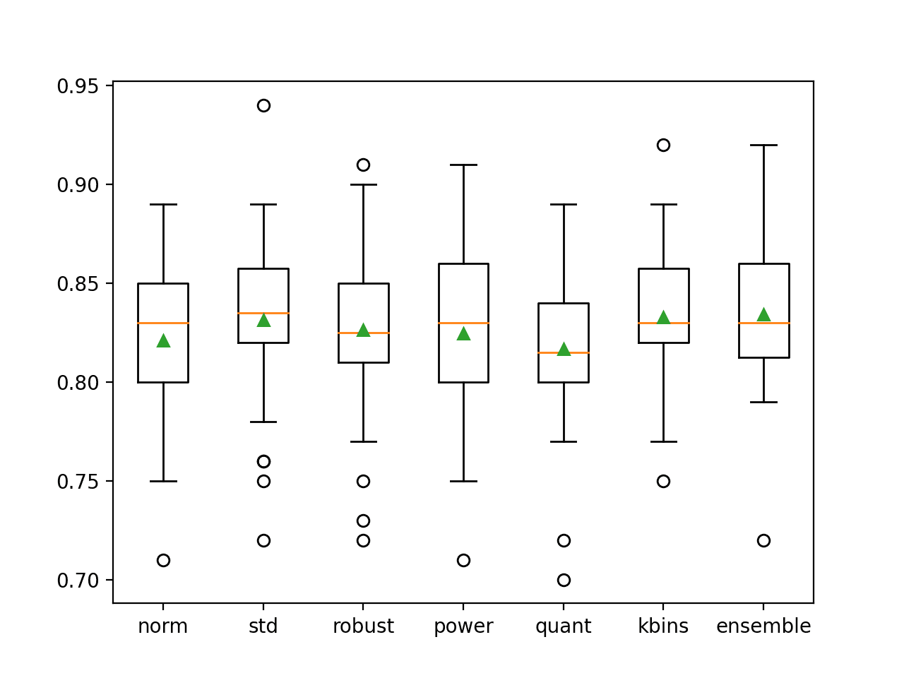
Box and Whisker Plot of Accuracy Distribution for Individual Models and Data Transform Ensemble
Now that we are familiar with how to develop a data transform ensemble for classification, let’s look at doing the same for regression.
Data Transform Ensemble for Regression
In this section, we will explore developing a data transform ensemble for a regression predictive modeling problem.
First, we can define a synthetic binary regression dataset as the basis for exploring this type of ensemble.
The example below creates a dataset with 1,000 examples each of 100 input features where 10 of them contain information for predicting the target.
|
1 2 3 4 5 6 |
# synthetic regression dataset from sklearn.datasets import make_regression # define dataset X, y = make_regression(n_samples=1000, n_features=100, n_informative=10, noise=0.1, random_state=1) # summarize the dataset print(X.shape, y.shape) |
Running the example creates the dataset and confirms the data has the expected shape.
|
1 |
(1000, 100) (1000,) |
Next, we can establish a baseline in performance on the synthetic dataset by fitting and evaluating the base model that we intend to use in the ensemble, in this case, a DecisionTreeRegressor.
The model will be evaluated using repeated k-fold cross-validation with three repeats and 10 folds. Model performance on the dataset will be reported using the mean absolute error, or MAE. The scikit-learn will invert the score (make it negative) so that the framework can maximize the score. As such, we can ignore the sign on the score.
The example below evaluates the decision tree on the synthetic regression dataset.
|
1 2 3 4 5 6 7 8 9 10 11 12 13 14 15 16 17 |
# evaluate decision tree on synthetic regression dataset from numpy import mean from numpy import std from sklearn.datasets import make_regression from sklearn.model_selection import cross_val_score from sklearn.model_selection import RepeatedKFold from sklearn.tree import DecisionTreeRegressor # define dataset X, y = make_regression(n_samples=1000, n_features=100, n_informative=10, noise=0.1, random_state=1) # define the model model = DecisionTreeRegressor() # define the evaluation procedure cv = RepeatedKFold(n_splits=10, n_repeats=3, random_state=1) # evaluate the model n_scores = cross_val_score(model, X, y, scoring='neg_mean_absolute_error', cv=cv, n_jobs=-1) # report performance print('MAE: %.3f (%.3f)' % (mean(n_scores), std(n_scores))) |
Running the example reports the MAE of the decision tree on the synthetic regression dataset.
Note: Your results may vary given the stochastic nature of the algorithm or evaluation procedure, or differences in numerical precision. Consider running the example a few times and compare the average outcome.
In this case, we can see that the model achieved a MAE of about 139.817. This provides a floor in performance that we expect the ensemble model to improve upon.
|
1 |
MAE: -139.817 (12.449) |
Next, we can develop and evaluate the ensemble.
We will use the same data transforms from the previous section. The VotingRegressor will be used to combine the predictions, which is appropriate for regression problems.
The get_ensemble() function defined below creates the individual models and the ensemble model and combines all of the models as a list of tuples for evaluation.
|
1 2 3 4 5 6 7 8 9 10 11 12 13 14 15 16 17 18 19 20 21 22 23 24 25 26 |
# get a voting ensemble of models def get_ensemble(): # define the base models models = list() # normalization norm = Pipeline([('s', MinMaxScaler()), ('m', DecisionTreeRegressor())]) models.append(('norm', norm)) # standardization std = Pipeline([('s', StandardScaler()), ('m', DecisionTreeRegressor())]) models.append(('std', std)) # robust robust = Pipeline([('s', RobustScaler()), ('m', DecisionTreeRegressor())]) models.append(('robust', robust)) # power power = Pipeline([('s', PowerTransformer()), ('m', DecisionTreeRegressor())]) models.append(('power', power)) # quantile quant = Pipeline([('s', QuantileTransformer(n_quantiles=100, output_distribution='normal')), ('m', DecisionTreeRegressor())]) models.append(('quant', quant)) # kbins kbins = Pipeline([('s', KBinsDiscretizer(n_bins=20, encode='ordinal')), ('m', DecisionTreeRegressor())]) models.append(('kbins', kbins)) # define the voting ensemble ensemble = VotingRegressor(estimators=models) # return a list of tuples each with a name and model return models + [('ensemble', ensemble)] |
We can then call this function and evaluate each contributing modeling pipeline independently and compare the results to the ensemble of the pipelines.
Our expectation, as before, is that the ensemble results in a lift in performance over any individual model. If it does not, then the top-performing individual model should be chosen instead.
Tying this together, the complete example for evaluating a data transform ensemble for a regression dataset is listed below.
|
1 2 3 4 5 6 7 8 9 10 11 12 13 14 15 16 17 18 19 20 21 22 23 24 25 26 27 28 29 30 31 32 33 34 35 36 37 38 39 40 41 42 43 44 45 46 47 48 49 50 51 52 53 54 55 56 57 58 59 60 61 |
# comparison of data transform ensemble to each contributing member for regression from numpy import mean from numpy import std from sklearn.datasets import make_regression from sklearn.model_selection import cross_val_score from sklearn.model_selection import RepeatedKFold from sklearn.preprocessing import MinMaxScaler from sklearn.preprocessing import StandardScaler from sklearn.preprocessing import RobustScaler from sklearn.preprocessing import PowerTransformer from sklearn.preprocessing import QuantileTransformer from sklearn.preprocessing import KBinsDiscretizer from sklearn.tree import DecisionTreeRegressor from sklearn.ensemble import VotingRegressor from sklearn.pipeline import Pipeline from matplotlib import pyplot # get a voting ensemble of models def get_ensemble(): # define the base models models = list() # normalization norm = Pipeline([('s', MinMaxScaler()), ('m', DecisionTreeRegressor())]) models.append(('norm', norm)) # standardization std = Pipeline([('s', StandardScaler()), ('m', DecisionTreeRegressor())]) models.append(('std', std)) # robust robust = Pipeline([('s', RobustScaler()), ('m', DecisionTreeRegressor())]) models.append(('robust', robust)) # power power = Pipeline([('s', PowerTransformer()), ('m', DecisionTreeRegressor())]) models.append(('power', power)) # quantile quant = Pipeline([('s', QuantileTransformer(n_quantiles=100, output_distribution='normal')), ('m', DecisionTreeRegressor())]) models.append(('quant', quant)) # kbins kbins = Pipeline([('s', KBinsDiscretizer(n_bins=20, encode='ordinal')), ('m', DecisionTreeRegressor())]) models.append(('kbins', kbins)) # define the voting ensemble ensemble = VotingRegressor(estimators=models) # return a list of tuples each with a name and model return models + [('ensemble', ensemble)] # generate regression dataset X, y = make_regression(n_samples=1000, n_features=100, n_informative=10, noise=0.1, random_state=1) # get models models = get_ensemble() # evaluate each model results = list() for name,model in models: # define the evaluation method cv = RepeatedKFold(n_splits=10, n_repeats=3, random_state=1) # evaluate the model on the dataset n_scores = cross_val_score(model, X, y, scoring='neg_mean_absolute_error', cv=cv, n_jobs=-1) # report performance print('>%s: %.3f (%.3f)' % (name, mean(n_scores), std(n_scores))) results.append(n_scores) # plot the results for comparison pyplot.boxplot(results, labels=[n for n,_ in models], showmeans=True) pyplot.show() |
Running the example first reports the MAE of each individual model, ending with the performance of the ensemble that combines the models.
Note: Your results may vary given the stochastic nature of the algorithm or evaluation procedure, or differences in numerical precision. Consider running the example a few times and compare the average outcome.
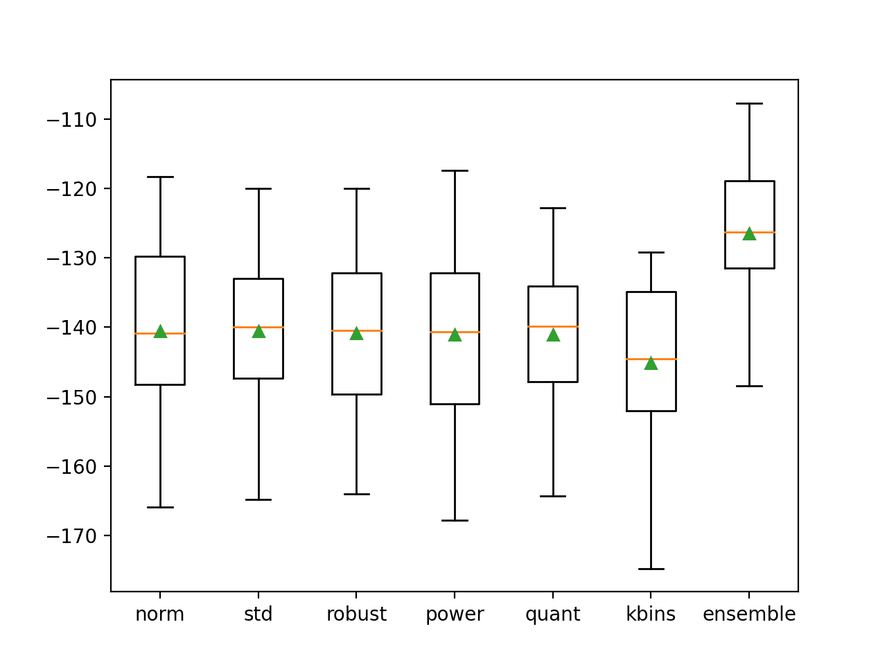
We can see that each model performs about the same, with MAE error scores around 140, all higher than the decision tree used in isolation. Interestingly, the ensemble performs the best, out-performing all of the individual members and the tree with no transforms, achieving a MAE of about 126.487.
This result suggests that although each pipeline performs worse than a single tree without transforms, each pipeline is making different errors and that the average of the models is able to leverage and harness these differences toward lower error.
|
1 2 3 4 5 6 7 |
>norm: -140.559 (11.783) >std: -140.582 (11.996) >robust: -140.813 (11.827) >power: -141.089 (12.668) >quant: -141.109 (11.097) >kbins: -145.134 (11.638) >ensemble: -126.487 (9.999) |
A figure is created comparing the distribution of MAE scores for each pipeline and the ensemble.
As we hoped, the distribution for the ensemble skews higher compared to all of the other models and has a higher (smaller) central tendency (mean and median indicated by the green triangle and orange line respectively).
Box and Whisker Plot of MAE Distributions for Individual Models and Data Transform Ensemble
Further Reading
This section provides more resources on the topic if you are looking to go deeper.
Tutorials
Books
- Pattern Classification Using Ensemble Methods, 2010.
- Ensemble Methods, 2012.
- Ensemble Machine Learning, 2012.
APIs
Summary
In this tutorial, you discovered how to develop a data transform ensemble.
Specifically, you learned:
- Data transforms can be used as the basis for a bagging-type ensemble where the same model is trained on different views of a training dataset.
- How to develop a data transform ensemble for classification and confirm the ensemble performs better than any contributing member.
- How to develop and evaluate a data transform ensemble for regression predictive modeling.
Do you have any questions?
Ask your questions in the comments below and I will do my best to answer.
Get a Handle on Modern Ensemble Learning!

Improve Your Predictions in Minutes
...with just a few lines of python code
Discover how in my new Ebook:
Ensemble Learning Algorithms With Python
It provides self-study tutorials with full working code on:
Stacking, Voting, Boosting, Bagging, Blending, Super Learner,
and much more...


Can we use this for sequence prediction (regression) problems where we have less number of features
I don’t see why not.
Dear Dr. Jason,
Thank you for the tutorial.
I tried to experiment with estimators with the housing dataset and found out that the best result was achieved with xgboost regressor on unseen data instead of decision trees. PolynomialFeatures() as an additional transformer also improves the score.
You’re welcome.
Nice work!
Thank you very much. This was awesome.
You’re welcome!
Dear Dr. Jason
Can I use this way for the data transformer that I write?
I have the data from stock and want to run this way for different technical indicator the create from data
Hi Mehdi…In theory there would be no issue. Please clarify the goals of your model so that we may better assist you.