A modeling averaging ensemble combines the prediction from each model equally and often results in better performance on average than a given single model.
Sometimes there are very good models that we wish to contribute more to an ensemble prediction, and perhaps less skillful models that may be useful but should contribute less to an ensemble prediction. A weighted average ensemble is an approach that allows multiple models to contribute to a prediction in proportion to their trust or estimated performance.
In this tutorial, you will discover how to develop a weighted average ensemble of deep learning neural network models in Python with Keras.
After completing this tutorial, you will know:
Model averaging ensembles are limited because they require that each ensemble member contribute equally to predictions.
Weighted average ensembles allow the contribution of each ensemble member to a prediction to be weighted proportionally to the trust or performance of the member on a holdout dataset.
How to implement a weighted average ensemble in Keras and compare results to a model averaging ensemble and standalone models.
Kick-start your project with my new book Better Deep Learning, including step-by-step tutorials and the Python source code files for all examples.
Let’s get started.
Updated Oct/2019: Updated for Keras 2.3 and TensorFlow 2.0.
Updated Jan/2020: Updated for changes in scikit-learn v0.22 API.
How to Develop a Weighted Average Ensemble for Deep Learning Neural Networks Photo by Simon Matzinger, some rights reserved.
Tutorial Overview
This tutorial is divided into six parts; they are:
Weighted Average Ensemble
Multi-Class Classification Problem
Multilayer Perceptron Model
Model Averaging Ensemble
Grid Search Weighted Average Ensemble
Optimized Weighted Average Ensemble
Weighted Average Ensemble
Model averaging is an approach to ensemble learning where each ensemble member contributes an equal amount to the final prediction.
In the case of regression, the ensemble prediction is calculated as the average of the member predictions. In the case of predicting a class label, the prediction is calculated as the mode of the member predictions. In the case of predicting a class probability, the prediction can be calculated as the argmax of the summed probabilities for each class label.
A limitation of this approach is that each model has an equal contribution to the final prediction made by the ensemble. There is a requirement that all ensemble members have skill as compared to random chance, although some models are known to perform much better or much worse than other models.
A weighted ensemble is an extension of a model averaging ensemble where the contribution of each member to the final prediction is weighted by the performance of the model.
The model weights are small positive values and the sum of all weights equals one, allowing the weights to indicate the percentage of trust or expected performance from each model.
One can think of the weight Wk as the belief in predictor k and we therefore constrain the weights to be positive and sum to one.
Uniform values for the weights (e.g. 1/k where k is the number of ensemble members) means that the weighted ensemble acts as a simple averaging ensemble. There is no analytical solution to finding the weights (we cannot calculate them); instead, the value for the weights can be estimated using either the training dataset or a holdout validation dataset.
Finding the weights using the same training set used to fit the ensemble members will likely result in an overfit model. A more robust approach is to use a holdout validation dataset unseen by the ensemble members during training.
The simplest, perhaps most exhaustive approach would be to grid search weight values between 0 and 1 for each ensemble member. Alternately, an optimization procedure such as a linear solver or gradient descent optimization can be used to estimate the weights using a unit norm weight constraint to ensure that the vector of weights sum to one.
Unless the holdout validation dataset is large and representative, a weighted ensemble has an opportunity to overfit as compared to a simple averaging ensemble.
A simple alternative to adding more weight to a given model without calculating explicit weight coefficients is to add a given model more than once to the ensemble. Although less flexible, it allows a given well-performing model to contribute more than once to a given prediction made by the ensemble.
Want Better Results with Deep Learning?
Take my free 7-day email crash course now (with sample code).
Click to sign-up and also get a free PDF Ebook version of the course.
Multi-Class Classification Problem
We will use a small multi-class classification problem as the basis to demonstrate the weighted averaging ensemble.
The scikit-learn class provides the make_blobs() function that can be used to create a multi-class classification problem with the prescribed number of samples, input variables, classes, and variance of samples within a class.
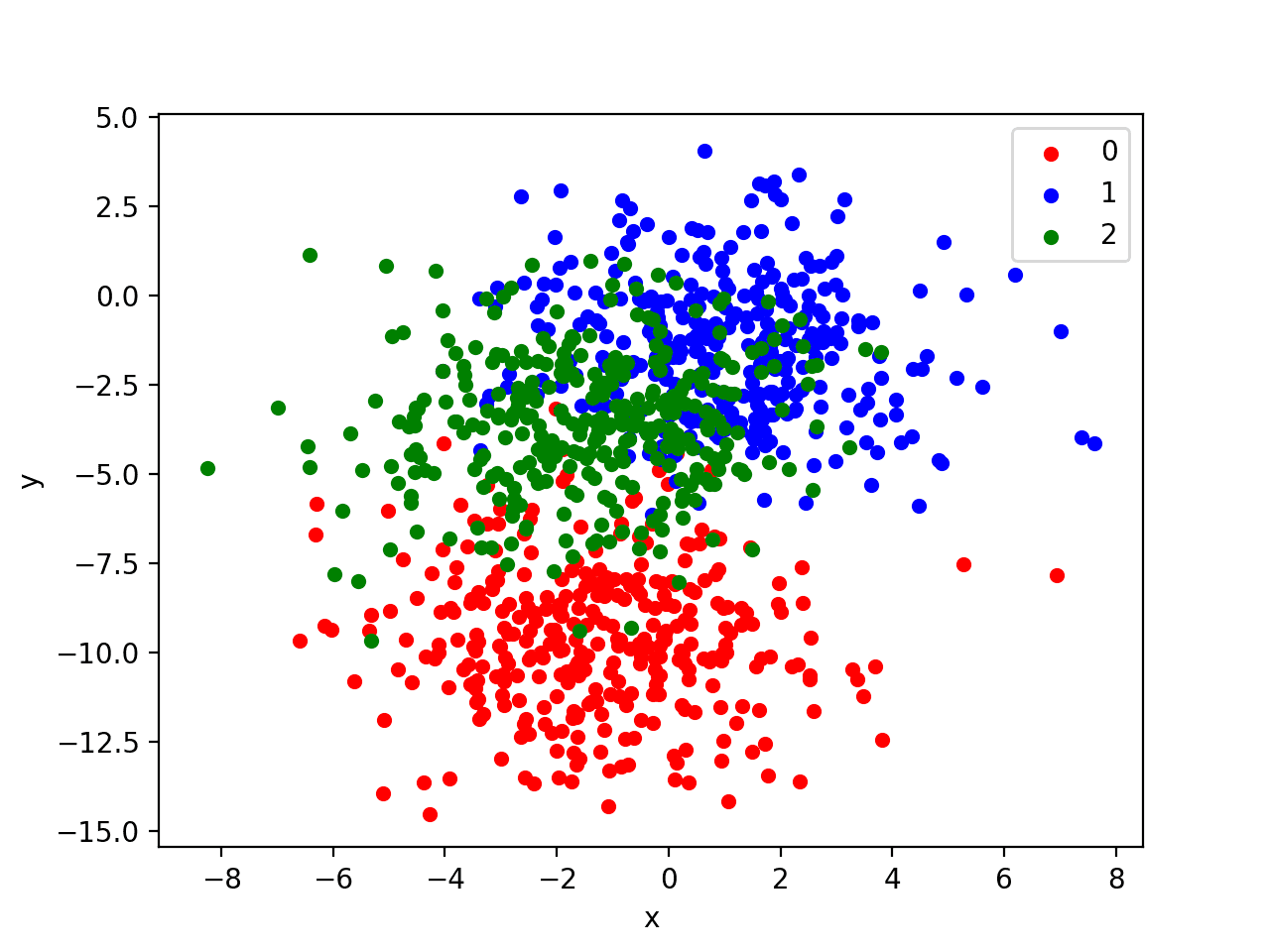
The problem has two input variables (to represent the x and y coordinates of the points) and a standard deviation of 2.0 for points within each group. We will use the same random state (seed for the pseudorandom number generator) to ensure that we always get the same data points.
The results are the input and output elements of a dataset that we can model.
In order to get a feeling for the complexity of the problem, we can plot each point on a two-dimensional scatter plot and color each point by class value.
Running the example creates a scatter plot of the entire dataset. We can see that the standard deviation of 2.0 means that the classes are not linearly separable (separable by a line) causing many ambiguous points.
This is desirable as it means that the problem is non-trivial and will allow a neural network model to find many different “good enough” candidate solutions resulting in a high variance.
Scatter Plot of Blobs Dataset With Three Classes and Points Colored by Class Value
Multilayer Perceptron Model
Before we define a model, we need to contrive a problem that is appropriate for the weighted average ensemble.
In our problem, the training dataset is relatively small. Specifically, there is a 10:1 ratio of examples in the training dataset to the holdout dataset. This mimics a situation where we may have a vast number of unlabeled examples and a small number of labeled examples with which to train a model.
We will create 1,100 data points from the blobs problem. The model will be trained on the first 100 points and the remaining 1,000 will be held back in a test dataset, unavailable to the model.
The problem is a multi-class classification problem, and we will model it using a softmax activation function on the output layer. This means that the model will predict a vector with three elements with the probability that the sample belongs to each of the three classes. Therefore, we must one hot encode the class values before we split the rows into the train and test datasets. We can do this using the Keras to_categorical() function.
The model will expect samples with two input variables. The model then has a single hidden layer with 25 nodes and a rectified linear activation function, then an output layer with three nodes to predict the probability of each of the three classes and a softmax activation function.
Because the problem is multi-class, we will use the categorical cross entropy loss function to optimize the model and the efficient Adam flavor of stochastic gradient descent.
Running the example first prints the shape of each dataset for confirmation, then the performance of the final model on the train and test datasets.
Note: Your results may vary given the stochastic nature of the algorithm or evaluation procedure, or differences in numerical precision. Consider running the example a few times and compare the average outcome.
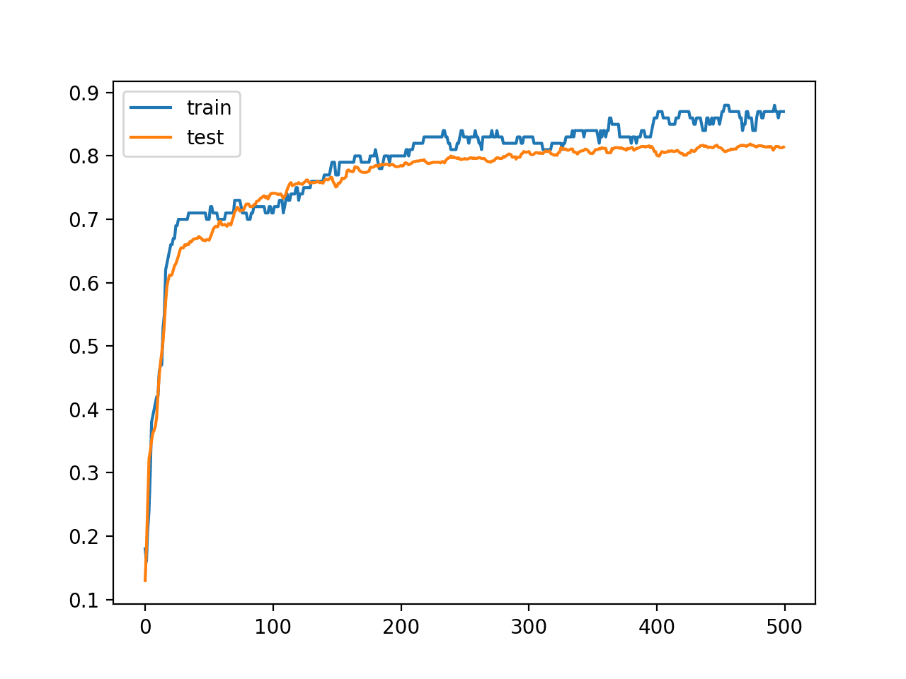
In this case, we can see that the model achieved about 87% accuracy on the training dataset, which we know is optimistic, and about 81% on the test dataset, which we would expect to be more realistic.
1
2
(100, 2) (1000, 2)
Train: 0.870, Test: 0.814
A line plot is also created showing the learning curves for the model accuracy on the train and test sets over each training epoch.
We can see that training accuracy is more optimistic over most of the run as we also noted with the final scores.
Line Plot Learning Curves of Model Accuracy on Train and Test Dataset over Each Training Epoch
Now that we have identified that the model is a good candidate for developing an ensemble, we can next look at developing a simple model averaging ensemble.
Model Averaging Ensemble
We can develop a simple model averaging ensemble before we look at developing a weighted average ensemble.
The results of the model averaging ensemble can be used as a point of comparison as we would expect a well configured weighted average ensemble to perform better.
First, we need to fit multiple models from which to develop an ensemble. We will define a function named fit_model() to create and fit a single model on the training dataset that we can call repeatedly to create as many models as we wish.
We don’t know how many members would be appropriate for this problem, so we can create ensembles with different sizes from one to 10 members and evaluate the performance of each on the test set.
We can also evaluate the performance of each standalone model in the performance on the test set. This provides a useful point of comparison for the model averaging ensemble, as we expect that the ensemble will out-perform a randomly selected single model on average.
Each model predicts the probabilities for each class label, e.g. has three outputs. A single prediction can be converted to a class label by using the argmax() function on the predicted probabilities, e.g. return the index in the prediction with the largest probability value. We can ensemble the predictions from multiple models by summing the probabilities for each class prediction and using the argmax() on the result. The ensemble_predictions() function below implements this behavior.
1
2
3
4
5
6
7
8
9
10
# make an ensemble prediction for multi-class classification
def ensemble_predictions(members,testX):
# make predictions
yhats=[model.predict(testX)formodel inmembers]
yhats=array(yhats)
# sum across ensemble members
summed=numpy.sum(yhats,axis=0)
# argmax across classes
result=argmax(summed,axis=1)
returnresult
We can estimate the performance of an ensemble of a given size by selecting the required number of models from the list of all models, calling the ensemble_predictions() function to make a prediction, then calculating the accuracy of the prediction by comparing it to the true values. The evaluate_n_members() function below implements this behavior.
1
2
3
4
5
6
7
8
# evaluate a specific number of members in an ensemble
The scores of the ensembles of each size can be stored to be plotted later, and the scores for each individual model are collected and the average performance reported.
1
2
3
4
5
6
7
8
9
10
11
12
13
14
# evaluate different numbers of ensembles on hold out set
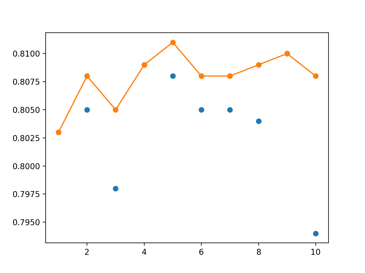
Finally, we create a graph that shows the accuracy of each individual model (blue dots) and the performance of the model averaging ensemble as the number of members is increased from one to 10 members (orange line).
Tying all of this together, the complete example is listed below.
Running the example first reports the performance of each single model as well as the model averaging ensemble of a given size with 1, 2, 3, etc. members.
Note: Your results may vary given the stochastic nature of the algorithm or evaluation procedure, or differences in numerical precision. Consider running the example a few times and compare the average outcome.
On this run, the average performance of the single models is reported at about 80.4% and we can see that an ensemble with between five and nine members will achieve a performance between 80.8% and 81%. As expected, the performance of a modest-sized model averaging ensemble out-performs the performance of a randomly selected single model on average.
1
2
3
4
5
6
7
8
9
10
11
12
(100, 2) (1000, 2)
> 1: single=0.803, ensemble=0.803
> 2: single=0.805, ensemble=0.808
> 3: single=0.798, ensemble=0.805
> 4: single=0.809, ensemble=0.809
> 5: single=0.808, ensemble=0.811
> 6: single=0.805, ensemble=0.808
> 7: single=0.805, ensemble=0.808
> 8: single=0.804, ensemble=0.809
> 9: single=0.810, ensemble=0.810
> 10: single=0.794, ensemble=0.808
Accuracy 0.804 (0.005)
Next, a graph is created comparing the accuracy of single models (blue dots) to the model averaging ensemble of increasing size (orange line).
On this run, the orange line of the ensembles clearly shows better or comparable performance (if dots are hidden) than the single models.
Line Plot Showing Single Model Accuracy (blue dots) and Accuracy of Ensembles of Increasing Size (orange line)
Now that we know how to develop a model averaging ensemble, we can extend the approach one step further by weighting the contributions of the ensemble members.
Grid Search Weighted Average Ensemble
The model averaging ensemble allows each ensemble member to contribute an equal amount to the prediction of the ensemble.
We can update the example so that instead, the contribution of each ensemble member is weighted by a coefficient that indicates the trust or expected performance of the model. Weight values are small values between 0 and 1 and are treated like a percentage, such that the weights across all ensemble members sum to one.
First, we must update the ensemble_predictions() function to make use of a vector of weights for each ensemble member.
Instead of simply summing the predictions across each ensemble member, we must calculate a weighted sum. We can implement this manually using for loops, but this is terribly inefficient; for example:
1
2
3
4
5
6
7
8
9
10
11
12
13
14
# calculated a weighted sum of predictions
def weighted_sum(weights,yhats):
rows=list()
forjinrange(yhats.shape[1]):
# enumerate values
row=list()
forkinrange(yhats.shape[2]):
# enumerate members
value=0.0
foriinrange(yhats.shape[0]):
value+=weights[i]*yhats[i,j,k]
row.append(value)
rows.append(row)
returnarray(rows)
Instead, we can use efficient NumPy functions to implement the weighted sum such as einsum() or tensordot().
Full discussion of these functions is a little out of scope so please refer to the API documentation for more information on how to use these functions as they are challenging if you are new to linear algebra and/or NumPy. We will use tensordot() function to apply the tensor product with the required summing; the updated ensemble_predictions() function is listed below.
1
2
3
4
5
6
7
8
9
10
# make an ensemble prediction for multi-class classification
def ensemble_predictions(members,weights,testX):
# make predictions
yhats=[model.predict(testX)formodel inmembers]
yhats=array(yhats)
# weighted sum across ensemble members
summed=tensordot(yhats,weights,axes=((0),(0)))
# argmax across classes
result=argmax(summed,axis=1)
returnresult
Next, we must update evaluate_ensemble() to pass along the weights when making the prediction for the ensemble.
1
2
3
4
5
6
# evaluate a specific number of members in an ensemble
Next, we can use a weight of 1/5 or 0.2 for each of the five ensemble members and use the new functions to estimate the performance of a model averaging ensemble, a so-called equal-weight ensemble.
We would expect this ensemble to perform as well or better than any single model.
Finally, we can develop a weighted average ensemble.
A simple, but exhaustive approach to finding weights for the ensemble members is to grid search values. We can define a course grid of weight values from 0.0 to 1.0 in steps of 0.1, then generate all possible five-element vectors with those values. Generating all possible combinations is called a Cartesian product, which can be implemented in Python using the itertools.product() function from the standard library.
A limitation of this approach is that the vectors of weights will not sum to one (called the unit norm), as required. We can force reach generated weight vector to have a unit norm by calculating the sum of the absolute weight values (called the L1 norm) and dividing each weight by that value. The normalize() function below implements this hack.
1
2
3
4
5
6
7
8
9
# normalize a vector to have unit norm
def normalize(weights):
# calculate l1 vector norm
result=norm(weights,1)
# check for a vector of all zeros
ifresult==0.0:
returnweights
# return normalized vector (unit norm)
returnweights/result
We can now enumerate each weight vector generated by the Cartesian product, normalize it, and evaluate it by making a prediction and keeping the best to be used in our final weight averaging ensemble.
1
2
3
4
5
6
7
8
9
10
11
12
13
14
15
16
17
18
# grid search weights
def grid_search(members,testX,testy):
# define weights to consider
w=[0.0,0.1,0.2,0.3,0.4,0.5,0.6,0.7,0.8,0.9,1.0]
best_score,best_weights=0.0,None
# iterate all possible combinations (cartesian product)
Once discovered, we can report the performance of our weight average ensemble on the test dataset, which we would expect to be better than the best single model and ideally better than the model averaging ensemble.
Running the example first creates the five single models and evaluates their performance on the test dataset.
Note: Your results may vary given the stochastic nature of the algorithm or evaluation procedure, or differences in numerical precision. Consider running the example a few times and compare the average outcome.
On this run, we can see that model 2 has the best solo performance of about 81.7% accuracy.
Next, a model averaging ensemble is created with a performance of about 80.7%, which is reasonable compared to most of the models, but not all.
1
2
3
4
5
6
7
(100, 2) (1000, 2)
Model 1: 0.798
Model 2: 0.817
Model 3: 0.798
Model 4: 0.806
Model 5: 0.810
Equal Weights Score: 0.807
Next, the grid search is performed. It is pretty slow and may take about twenty minutes on modern hardware. The process could easily be made parallel using libraries such as Joblib.
Each time a new top performing set of weights is discovered, it is reported along with its performance on the test dataset. We can see that during the run, the process discovered that using model 2 alone resulted in a good performance, until it was replaced with something better.
We can see that the best performance was achieved on this run using the weights that focus only on the first and second models with the accuracy of 81.8% on the test dataset. This out-performs both the single models and the model averaging ensemble on the same dataset.
An alternate approach to finding weights would be a random search, which has been shown to be effective more generally for model hyperparameter tuning.
Weighted Average MLP Ensemble
An alternative to searching for weight values is to use a directed optimization process.
Optimization is a search process, but instead of sampling the space of possible solutions randomly or exhaustively, the search process uses any available information to make the next step in the search, such as toward a set of weights that has lower error.
The SciPy library offers many excellent optimization algorithms, including local and global search methods.
SciPy provides an implementation of the Differential Evolution method. This is one of the few stochastic global search algorithms that “just works” for function optimization with continuous inputs, and it works well.
The differential_evolution() SciPy function requires that function is specified to evaluate a set of weights and return a score to be minimized. We can minimize the classification error (1 – accuracy).
As with the grid search, we most normalize the weight vector before we evaluate it. The loss_function() function below will be used as the evaluation function during the optimization process.
1
2
3
4
5
6
# loss function for optimization process, designed to be minimized
We must also specify the bounds of the optimization process. We can define the bounds as a five-dimensional hypercube (e.g. 5 weights for the 5 ensemble members) with values between 0.0 and 1.0.
1
2
# define bounds on each weight
bound_w=[(0.0,1.0)for_inrange(n_members)]
Our loss function requires three parameters in addition to the weights, which we will provide as a tuple to then be passed along to the call to the loss_function() each time a set of weights is evaluated.
1
2
# arguments to the loss function
search_arg=(members,testX,testy)
We can now call our optimization process.
We will limit the total number of iterations of the algorithms to 1,000, and use a smaller than default tolerance to detect if the search process has converged.
The result of the call to differential_evolution() is a dictionary that contains all kinds of information about the search.
Importantly, the ‘x‘ key contains the optimal set of weights found during the search. We can retrieve the best set of weights, then report them and their performance on the test set when used in a weighted ensemble.
Running the example first creates five single models and evaluates the performance of each on the test dataset.
Note: Your results may vary given the stochastic nature of the algorithm or evaluation procedure, or differences in numerical precision. Consider running the example a few times and compare the average outcome.
We can see on this run that models 3 and 4 both perform best with an accuracy of about 82.2%.
Next, a model averaging ensemble with all five members is evaluated on the test set reporting an accuracy of 81.8%, which is better than some, but not all, single models.
1
2
3
4
5
6
7
(100, 2) (1000, 2)
Model 1: 0.814
Model 2: 0.811
Model 3: 0.822
Model 4: 0.822
Model 5: 0.809
Equal Weights Score: 0.818
The optimization process is relatively quick.
We can see that the process found a set of weights that pays most attention to models 3 and 4, and spreads the remaining attention out among the other models, achieving an accuracy of about 82.4%, out-performing the model averaging ensemble and individual models.
It is important to note that in these examples, we have treated the test dataset as though it were a validation dataset. This was done to keep the examples focused and technically simpler. In practice, the choice and tuning of the weights for the ensemble would be chosen by a validation dataset, and single models, model averaging ensembles, and weighted ensembles would be compared on a separate test set.
Extensions
This section lists some ideas for extending the tutorial that you may wish to explore.
Parallelize Grid Search. Update the grid search example to use the Joblib library to parallelize weight evaluation.
Implement Random Search. Update the grid search example to use a random search of weight coefficients.
Try a Local Search. Try a local search procedure provided by the SciPy library instead of the global search and compare performance.
Repeat Global Optimization. Repeat the global optimization procedure multiple times for a given set of models to see if differing sets of weights can be found across the runs.
If you explore any of these extensions, I’d love to know.
Further Reading
This section provides more resources on the topic if you are looking to go deeper.
In this tutorial, you discovered how to develop a weighted average ensemble of deep learning neural network models in Python with Keras.
Specifically, you learned:
Model averaging ensembles are limited because they require that each ensemble member contribute equally to predictions.
Weighted average ensembles allow the contribution of each ensemble member to a prediction to be weighted proportionally to the trust or performance of the member on a holdout dataset.
How to implement a weighted average ensemble in Keras and compare results to a model averaging ensemble and standalone models.
Do you have any questions?
Ask your questions in the comments below and I will do my best to answer.
Additionally using models whose error terms are not correlated yield better results..
One query: some suggest giving weights inversely proportional to RMSE or directly proportional to accuracy measures. Do you find weights derived from this method are similar to the weights derived from grid search? Or do they differ?
Try Local Search with Scipy optimization library, initializing weight with the coefficients of a Linear, Ridge, or Lasso regression. It will only take a few seconds but will have similar performance as the grid search.
Great article,thanks Jason.
I have some concern with the weighted average ensemble. Will it worsen the overfitting problem?After all,machine learning algorithm is already prone to overfitting,now is giving the different models different weights another level of overfitting?Is it really better than the normal average weight version in the out-sample prediction?
“Your results will vary given the stochastic nature of the training algorithm.”
Which I don’t really understand as the make_blob function call makes use of random_state parameter, so it’s output should be deterministic. So I wonder where exactly the differences of the results come from?
Can we create a heterogeneous ensemble model using other classification algorithms like Gaussian Naive Bayes, KNN, etc., and still optimize weights using Differential Evolution
Hi,
While using another dataset after execution of this block
def ensemble_predictions(members, weights, x_test):
yhats = [model.predict(x_test) for model in members]
yhats = array(yhats)
# sum across ensemble members
summed = tensordot(yhats, weights, axes=((0),(0)))
# argmax across classes
result = argmax(summed, axis=1)
Hi great article, I have few concerns, no matter the stacking or ensemble method, the models should try to capture different aspects of data or predict different results before feeding to the ensemble, thus we can make huge difference on the accuracy not just based on the random seed on one algorithm.
This may seem like a dumb question, so excuse my ignorance, but I’m wondering if there’s a way to then save the weights to a single checkpoint file to use later? I see that we create 5 separate models during this process and getting 5 different accuracy scores, and I’m ok with saving those 5 different sets of weights as checkpoint files and then saving their accuracy scores to a file to refer to them again later, and then making forward predictions based on those score weights, but just wondering if there’s a way to combine them into one file to make things easier? Thanks again!
Hi Jason. Thanks for the tutorial. How can I approach the problem where I have two different models that takes two different inputs ? Suppose I have one LSTM model that takes time series data as input and another CNN model that takes word embedding vectors of text as input. So if I want to ensemble those two models based on the weighted average technique, how should the different input types be combined to get the optimized weights ? Can I also use the same optimization algorithm that you have used ?
I have learned a lot from this topic. I am a newbie and I have a doubt. Pardon me if it is dumb.
One thing that I’m confused is about the weighted average term. The code finds out the weighted majority of the predicted class through argmax function. Where is the weighted AVERAGE being calculated?
I would like to change the sentence in the previous query as “The code results in giving Predicted class for each instance by choosing the highest weighted sum using argmax function”.
Thanks
sir as i have applied grid search optimization to deep learning model.after that how i can apply ensemble technique for example i may apply grid search to all the base deep learning model or is there any other way to apply ensemble technique
Hi, my optimized weights seem not follows to the single model’s score as yours, although the final score of the ensemble model out-performs others. I retrain multiple times (The same code of yours):
Model 1: 0.815
Model 2: 0.809
Model 3: 0.818
Model 4: 0.808
Model 5: 0.806
Equal weights score: 0.814
Optimized Weights Score: [0.07226963 0.25272131 0.10460353 0.14405271 0.42635282]
Grid Search Weights: [0.07226963 0.25272131 0.10460353 0.14405271 0.42635282], Score: 0.818
Hi,
I really appreciate your hard work. I have a question here
I have used a model average ensemble code ( with some changes for regression task) , now I want to compare my model with grid search weighted average ensemble model for regression application. But I am stuck at the tensordot function.
Can you please give me a hint that how can I use that function in regression application?
Thanks for your reply. I have prepared weighted average ensemble for my regression problem.
My question is when I am taking n_members upto 4 then there is no problem but when I am taking n_members >=5 then the model is keep running for several hours neither giving any error nor giving final best weights. Do you have any idea what can be the reason behind it?
Yes, there is no bug because when I am initializing weights by w= [0,0.5,1] then the model is normally running for n_members=5 but for higher n_members around >=8 again it is neither giving any error nor final best weights.
I think the reason may be the complex model for higher n_members?
Thank you so much for writing great articles with great explanation.
I have a question, that what would be our final model in this case which will go in production? In meta learning (stacking generalization) we do have final model at the end, but in this case what would be our final model to put in production?
How would you make an ensemble of models that have different input shapes due to different window size, such as LSTM models. So the input shapes for Model A would be (window_size_A, features) and for Model B would be (window_size_B, features). The window sizes are different but the number of features are the same. As such, due to the different window size, the training data of the same dataset is split differently for each model such that the X_train.shape for model A: (train_data_A, window_size_A, output) And for Model B: (train_data_B, window_size_B, output). Note the training data is from the same dataset but the length is different due to the different window size. The number of outputs is the same for Model A and Model B. How would you make an ensemble of these models?
For example, how would you make an ensemble of these 2 models, specifically in terms of accommodating the different window sizes i.e. input shapes? As the input shapes for the models in your post are all the same.
Thank you for this suggestion and for the recommended article. I tried making a multi-input model and then having a different shape for the training data of each model I.e. for model A: (samples_A, window_size_A, features) and for model B: (samples_B, window_size_B, features). The size of samples_A and samples_B are different due to different window sizes. But now the shape of the training data is different and so is the shape of the validation and testing data. So you can train model A on training set A I.e.(trainsamples_A, window_size_A, features), and then compare to validation set A I.e.(validationsamples_A, window_size_A, features) and test model A on the test set I.e.(testsamples_A, window_size_A, features); and do the same for model B. But when combining the models, what do you test the ensemble on? What should be the test shape? Because the test shape for models A and model B are determined by their window size.
Thank you. I understand and agree with you, that each input model can have a separate train and validation set. But once combined, to make the ensemble model, what test set, should the ensemble model be tested on? Because the test set for both the input models are a different shape due to the different window size. Each individual input model can be tested on it’s own test set, but what about the completed ensemble model?
models = [firstmodel, secondmodel]
def ensemble(models, model_input):
outputs = [model.outputs[0] for model in models]
y = Average()(outputs)
model = Model(inputs = model_input, outputs = y, name=”ensemble”)
return model
What will be the model_input for the ensemble model then? Also what will the shape of X_test be for the ensemble model? Because when there was only one input, like the first_model_input = Input(shape=(50,2)) then the X_test.shape was (2554, 50, 2).
But now there are two inputs, so there are two X_test shapes, one for first model input which is (2554, 50, 2) and one for the second model input which is (2544, 60, 2).
I’m still stuck with the same problem but might try with a contrived dataset now.
I was wondering, why not ensemble different models by training a simple fully connected network (its inputs being the predictions from each model)? I feel like a weighted average is a simple linear behaviour and non-linearity might imporve performance. Is it because it is much simpler to interpret a weighted average or there is more to it?
How to save the weighted ensemble model as a new model for later prediction, like new_model.predict(X_test)?
In addition, when we do differential_evolution(), we call ensemble_predictions(members, weights, testX) many many times. If each trained model is a relatively complex one, model.predict() will take quite an amount of time. Actually, we only need to get yhats once I think. So how about we add one def to calculate yhats (def calculat_yhats(members, testX):, return yhats), then call ensemble_predictions(yhats, weights, testX).
I am not very sure if we need to calculate yhats every time when we optimize weights. Based on my understanding, we only need once. Please correct me if I am wrong. Thank you very much
If the sub-model does not change, then the predictions made by the model do not need to be re-calculated when optimizing the weights that combine those predictions.
Sorry for my stupid question in advance, i am struggling with tensordot fucntion, how do you multiply “yhats” with a weighted vector? its giving me ValueError: shape mismatch for sum of tensordot.


Great article Jason! Thank you..
Additionally using models whose error terms are not correlated yield better results..
One query: some suggest giving weights inversely proportional to RMSE or directly proportional to accuracy measures. Do you find weights derived from this method are similar to the weights derived from grid search? Or do they differ?
Thanks in advance Jason.
I prefer to use a global optimization algorithm to find robust weights.
Hi Jason, nice write-up, thanks for sharing!
Try Local Search with Scipy optimization library, initializing weight with the coefficients of a Linear, Ridge, or Lasso regression. It will only take a few seconds but will have similar performance as the grid search.
Great suggestion, do you think it would out-perform a global search like DE though?
I’m skeptical as I think the error surface is highly non-linear and probably multi-modal.
Very nice example.
Thanks,
Jay
Thanks Jay.
Great article,thanks Jason.
I have some concern with the weighted average ensemble. Will it worsen the overfitting problem?After all,machine learning algorithm is already prone to overfitting,now is giving the different models different weights another level of overfitting?Is it really better than the normal average weight version in the out-sample prediction?
It is a risk, but the risk can be lessened by using a separate validation dataset or out of sample data to fit the weights.
Hi
The article says:
“Your results will vary given the stochastic nature of the training algorithm.”
Which I don’t really understand as the make_blob function call makes use of random_state parameter, so it’s output should be deterministic. So I wonder where exactly the differences of the results come from?
Thanks
The differences come from the stochastic initialization and training of the model/s.
Hi Jason,
As always I find a solution to a problem that I have, in your article. Thank you .
Can the DE implementation be done using only sklearn and not keras. If so can you please suggest a resource on that?.
As far as I know sklearn does not have a DE implementation.
Thanks for the quick response.
Can we create a heterogeneous ensemble model using other classification algorithms like Gaussian Naive Bayes, KNN, etc., and still optimize weights using Differential Evolution
Sure, you might want to combine sklearn models with neural nets.
This would be a stacking ensemble:
https://machinelearningmastery.com/stacking-ensemble-for-deep-learning-neural-networks/
Hi,
While using another dataset after execution of this block
def ensemble_predictions(members, weights, x_test):
yhats = [model.predict(x_test) for model in members]
yhats = array(yhats)
# sum across ensemble members
summed = tensordot(yhats, weights, axes=((0),(0)))
# argmax across classes
result = argmax(summed, axis=1)
I get the following error:
~\Anaconda3\lib\site-packages\numpy\core\fromnumeric.py in argmax(a, axis, out)
961
962 “””
–> 963 return _wrapfunc(a, ‘argmax’, axis=axis, out=out)
964
965
~\Anaconda3\lib\site-packages\numpy\core\fromnumeric.py in _wrapfunc(obj, method, *args, **kwds)
55 def _wrapfunc(obj, method, *args, **kwds):
56 try:
—> 57 return getattr(obj, method)(*args, **kwds)
AxisError: axis 1 is out of bounds for array of dimension 1
Can you please suggest a solution to get rid of this.
Thank you.
Perhaps check that your dataset was loaded correctly and the model was suitable modified to account for the number of features in your dataset.
Thank You, Jason. I checked and got the individual performance accuracy of 4 models.
Can you please show how the output should look like after execution of the code below.
>>summed = tensordot(yhats, weights, axes=((0),(0))) #summed = np.sum(yhats, axis=0)
>>print(“summed”,summed)
After summing up equal weights(0.25) with the predicted result yhats for 4 models I am getting something like this
summed [ 1.5 0.5 2. 1. 1. 2. 1.25 1.25 1. 1.5 0. 1. 2.
0. 1.75 1. 0.5 0.5 1. 2. 1.25 1.5 0. 0.5 1.75
1. 0. 0. 1. 0. 1. 0. 2. 1. 1. 1.5 2. 1.
1. 1. 1. 1. 1. 2. 1. 1. 1. 2. 1.25 1. 1.
2. 1.5 0.5 1. 0. 1. 1. 0.5 1.5 0. 0. 0.
1.25 0. 1. 1.25 0. 2. 0.5 2. 1.25 0.5 1. 2. 0.5
2. 0.5 1. 2. 1.5 2. 0. 1.5 1.25 2. 1.5 1.25
1.5 1.75 0. 1. 1. 2. 1.5 0. ]
Is this correct?
Sorry, I cannot run or debug modified versions of the tutorial for tutorial for you.
The Shape of X_train and X_test is (384, 16) (96, 16) respectively
Did you ever figure this out? I have the same issue you with “AxisError: axis 1 is out of bounds for array of dimension 1” on the “summed” array.
Sent the next text before noticing your response.
I just wanted to know if the structure after summing of weights should look like this.
Never mind. I shall try.
Thank you for your prompt reply.
Hi great article, I have few concerns, no matter the stacking or ensemble method, the models should try to capture different aspects of data or predict different results before feeding to the ensemble, thus we can make huge difference on the accuracy not just based on the random seed on one algorithm.
Yes.
Hi Jason,
Very informative article.
How to convert the ensemble create to be used with a fit method without loop like this
ensemble.fit ?
Thanks.
There is no ensemble.fit.
Hi Jason,
Is there any default value for mutation and crossover parameter in the DifferentialEvolution method used here? or is it ok to not uses these.
Yes and the defaults work well.
The details are here:
https://docs.scipy.org/doc/scipy/reference/generated/scipy.optimize.differential_evolution.html
Hi, nice work, a bug should be changed, the line “y = to_categorical(y)”, this will change y many times if y always exists in memory, like in jupyter
Thanks, but the script is designed to be run once from the command line.
Thanks William, as a newbie i’ve been confused for almost a day
Hi, How can we use this procedure for regression problem?
Thanks
You can adapt the example for regression. I don’t have a worked example at this stage.
hi Branda, please guide me to develop a ensemble model for regression problem?
Awesome! Another thing for me to play with!
This may seem like a dumb question, so excuse my ignorance, but I’m wondering if there’s a way to then save the weights to a single checkpoint file to use later? I see that we create 5 separate models during this process and getting 5 different accuracy scores, and I’m ok with saving those 5 different sets of weights as checkpoint files and then saving their accuracy scores to a file to refer to them again later, and then making forward predictions based on those score weights, but just wondering if there’s a way to combine them into one file to make things easier? Thanks again!
Disregard my last! I found another article on your site that answers my question found here :
https://machinelearningmastery.com/polyak-neural-network-model-weight-ensemble/
Thanks!
No problem.
Yes, you can save a model via the save() function:
https://machinelearningmastery.com/save-load-keras-deep-learning-models/
You can save an array of weights to file:
https://machinelearningmastery.com/how-to-save-a-numpy-array-to-file-for-machine-learning/
Hi Jason. Thanks for the tutorial. How can I approach the problem where I have two different models that takes two different inputs ? Suppose I have one LSTM model that takes time series data as input and another CNN model that takes word embedding vectors of text as input. So if I want to ensemble those two models based on the weighted average technique, how should the different input types be combined to get the optimized weights ? Can I also use the same optimization algorithm that you have used ?
You weight their predictions (outputs), not their inputs.
In that sense, their inputs do not matter.
Hi Jason,
I have learned a lot from this topic. I am a newbie and I have a doubt. Pardon me if it is dumb.
One thing that I’m confused is about the weighted average term. The code finds out the weighted majority of the predicted class through argmax function. Where is the weighted AVERAGE being calculated?
Please clarify my doubt.
Thank you.
I would like to change the sentence in the previous query as “The code results in giving Predicted class for each instance by choosing the highest weighted sum using argmax function”.
Thanks
We weight the contribution of each models prediction to a final prediction, then convert the prediction to a class label.
Thank You for the response. But my doubt is about averaging . Where does averaging happen? excuse my dumbness
We use a sum of the predicted probabilities for each class label, the average is just a normalized sum.
sir as i have applied grid search optimization to deep learning model.after that how i can apply ensemble technique for example i may apply grid search to all the base deep learning model or is there any other way to apply ensemble technique
Typically you don’t want highly tuned models in an ensemble, it can make the ensemble unstable/fragile.
You want “good enough” models in the ensemble.
Hi, my optimized weights seem not follows to the single model’s score as yours, although the final score of the ensemble model out-performs others. I retrain multiple times (The same code of yours):
Model 1: 0.815
Model 2: 0.809
Model 3: 0.818
Model 4: 0.808
Model 5: 0.806
Equal weights score: 0.814
Optimized Weights Score: [0.07226963 0.25272131 0.10460353 0.14405271 0.42635282]
Grid Search Weights: [0.07226963 0.25272131 0.10460353 0.14405271 0.42635282], Score: 0.818
Do you have any idea???
Yes, see this:
https://machinelearningmastery.com/faq/single-faq/why-do-i-get-different-results-each-time-i-run-the-code
Hi,
I really appreciate your hard work. I have a question here
I have used a model average ensemble code ( with some changes for regression task) , now I want to compare my model with grid search weighted average ensemble model for regression application. But I am stuck at the tensordot function.
Can you please give me a hint that how can I use that function in regression application?
Thanks.
I believe it would be the same, without the argmax.
Thanks for your reply. I have prepared weighted average ensemble for my regression problem.
My question is when I am taking n_members upto 4 then there is no problem but when I am taking n_members >=5 then the model is keep running for several hours neither giving any error nor giving final best weights. Do you have any idea what can be the reason behind it?
Perhaps confirm that you did not introduce a bug?
Yes, there is no bug because when I am initializing weights by w= [0,0.5,1] then the model is normally running for n_members=5 but for higher n_members around >=8 again it is neither giving any error nor final best weights.
I think the reason may be the complex model for higher n_members?
Sorry, I do not know the cause of the fault.
Perhaps you are running out of RAM?
Hi Jason,
Thank you so much for writing great articles with great explanation.
I have a question, that what would be our final model in this case which will go in production? In meta learning (stacking generalization) we do have final model at the end, but in this case what would be our final model to put in production?
Thank you so much!
You’re welcome.
The final model is the ensemble of models.
How would you make an ensemble of models that have different input shapes due to different window size, such as LSTM models. So the input shapes for Model A would be (window_size_A, features) and for Model B would be (window_size_B, features). The window sizes are different but the number of features are the same. As such, due to the different window size, the training data of the same dataset is split differently for each model such that the X_train.shape for model A: (train_data_A, window_size_A, output) And for Model B: (train_data_B, window_size_B, output). Note the training data is from the same dataset but the length is different due to the different window size. The number of outputs is the same for Model A and Model B. How would you make an ensemble of these models?
For example, how would you make an ensemble of these 2 models, specifically in terms of accommodating the different window sizes i.e. input shapes? As the input shapes for the models in your post are all the same.
Model1:
inputA= Input(shape(window_size_A, features))
hiddenA1=LSTM(units_A1, return_sequences=True)(inputA)
hiddenA2 = LSTM(units_A2, activation= ‘relu’)(hiddenA1) predictionA = Dense(output_A)(hiddenA2)
Model2:
inputB= Input(shape(window_size_B, features))
hiddenB1=LSTM(units_B1, return_sequences=True)(inputB)
hiddenB2 = LSTM(units_B2, activation= ‘relu’)(hiddenB1) prediction = Dense(output_B)(hiddenB2)
I’d really appreciate your advice in this matter.
Maybe a multi-input model with separate training data for each input “model”.
This will help:
https://machinelearningmastery.com/keras-functional-api-deep-learning/
Thank you for this suggestion and for the recommended article. I tried making a multi-input model and then having a different shape for the training data of each model I.e. for model A: (samples_A, window_size_A, features) and for model B: (samples_B, window_size_B, features). The size of samples_A and samples_B are different due to different window sizes. But now the shape of the training data is different and so is the shape of the validation and testing data. So you can train model A on training set A I.e.(trainsamples_A, window_size_A, features), and then compare to validation set A I.e.(validationsamples_A, window_size_A, features) and test model A on the test set I.e.(testsamples_A, window_size_A, features); and do the same for model B. But when combining the models, what do you test the ensemble on? What should be the test shape? Because the test shape for models A and model B are determined by their window size.
Any insight would be much appreciated.
Should not be a problem as each input model can take a separate train and validation dataset array/matrix.
Thank you. I understand and agree with you, that each input model can have a separate train and validation set. But once combined, to make the ensemble model, what test set, should the ensemble model be tested on? Because the test set for both the input models are a different shape due to the different window size. Each individual input model can be tested on it’s own test set, but what about the completed ensemble model?
Appreciate all your guidance thus far!
You would test it on data not used to train the model prepared in a way required for each input model.
If this is challenging for you – perhaps develop some prototypes with contrived data to get used to or learn more about the data preparation step.
Thank you again. I think the problem might be data preparation.
I managed lstm ensemble with one model input for each of the lstm models and for the ensemble model and it works perfectly for just one.
model_input = Input(shape=(50,2))
def firstmodel(model_input):
hiddenA1 = LSTM(6, return_sequences=True)(model_input)
hiddenA2 = LSTM(4, activation=’relu’)(hiddenA1)
outputA = Dense(24)(hiddenA2)
model = Model(inputs= model_input, outputs= outputA, name=”firstmodel”)
return model
def secondmodel(model_input):
hiddenB1 = LSTM(30, return_sequences=True)(model_input)
hiddenB2 = LSTM(20, activation=’relu’)(hiddenB1)
outputB = Dense(24)(hiddenB2)
model = Model(inputs= model_input, outputs= outputB, name=”secondmodel”)
return model
firstmodel = firstmodel(model_input)
secondmodel = secondmodel(model_input)
models = [firstmodel, secondmodel]
def ensemble(models, model_input):
outputs = [model.outputs[0] for model in models]
y = Average()(outputs)
model = Model(inputs = model_input, outputs = y, name=”ensemble”)
return model
ensemblemodel = (models, model_input)
def evaluate_rmse(model):
pred = model.predict(X_test)
rmse = np.sqrt(mean_squared_error(y_test, pred))
return rmse
ensemble_rmse = evaluate_rmse(ensemblemodel)
But what happens when there are two different model inputs for the first and second model:
first_model_input = Input(shape=(50,2))
second_model_input = Input(shape=(60,2))
What will be the model_input for the ensemble model then? Also what will the shape of X_test be for the ensemble model? Because when there was only one input, like the first_model_input = Input(shape=(50,2)) then the X_test.shape was (2554, 50, 2).
But now there are two inputs, so there are two X_test shapes, one for first model input which is (2554, 50, 2) and one for the second model input which is (2544, 60, 2).
I’m still stuck with the same problem but might try with a contrived dataset now.
Sorry to hear that you’re having trouble, perhaps some of these tops will help:
https://machinelearningmastery.com/faq/single-faq/can-you-read-review-or-debug-my-code
Thank you ????❤
You’re welcome.
i wanted to know how do i speed up the differential evolution optimization, it is running but taking way too long
Great question!
Perhaps try a simpler objective function?
Perhaps try few population members?
Perhaps try running on a faster CPU?
I am actually working on a colab notebook, and I have reduced the members as well but still taking way too long
Perhaps try on a large AWS EC2 instance?
ohok! thank you! 🙂
You’re welcome.
Hi Jason, thanks for your awesome tutorials.
I was wondering, why not ensemble different models by training a simple fully connected network (its inputs being the predictions from each model)? I feel like a weighted average is a simple linear behaviour and non-linearity might imporve performance. Is it because it is much simpler to interpret a weighted average or there is more to it?
Yes, you can do that. Sounds like a “stacking” ensemble:
https://machinelearningmastery.com/stacking-ensemble-for-deep-learning-neural-networks/
Thanks for the reference. And thanks again for all the work you do!
You’re welcome.
a maximum number of models in an ensemble model?
No maximum.
At some point, you will reach diminishing returns.
Thank you so much for your great article.
How to save the weighted ensemble model as a new model for later prediction, like new_model.predict(X_test)?
In addition, when we do differential_evolution(), we call ensemble_predictions(members, weights, testX) many many times. If each trained model is a relatively complex one, model.predict() will take quite an amount of time. Actually, we only need to get yhats once I think. So how about we add one def to calculate yhats (def calculat_yhats(members, testX):, return yhats), then call ensemble_predictions(yhats, weights, testX).
I am not very sure if we need to calculate yhats every time when we optimize weights. Based on my understanding, we only need once. Please correct me if I am wrong. Thank you very much
You’re welcome.
Perhaps you can save each neural net model and then save the weightings.
Thank you very much. Could you please answer my second question about if I only need to calculate yhats once?
If the sub-model does not change, then the predictions made by the model do not need to be re-calculated when optimizing the weights that combine those predictions.
Thank you! In your example, I think that we only need to do model.predict() once.
You’re welcome.
Amazing article Jason, thanks.
Saying so, the weighted average is not a good idea in LOOCV approach right?
Why is that?
Sorry for my stupid question in advance, i am struggling with tensordot fucntion, how do you multiply “yhats” with a weighted vector? its giving me ValueError: shape mismatch for sum of tensordot.
Perhaps you can start with the working example above and slowly adapt it for your specific example.
Or Perhaps you can multiple the predictions by the weights manually in a for loop.
Thank you so much sir, the problem has been solved
I’m happy to hear that.