Deep learning neural networks learn a mapping function from inputs to outputs.
This is achieved by updating the weights of the network in response to the errors the model makes on the training dataset. Updates are made to continually reduce this error until either a good enough model is found or the learning process gets stuck and stops.
The process of training neural networks is the most challenging part of using the technique in general and is by far the most time consuming, both in terms of effort required to configure the process and computational complexity required to execute the process.
In this post, you will discover the challenge of finding model parameters for deep learning neural networks.
After reading this post, you will know:
- Neural networks learn a mapping function from inputs to outputs that can be summarized as solving the problem of function approximation.
- Unlike other machine learning algorithms, the parameters of a neural network must be found by solving a non-convex optimization problem with many good solutions and many misleadingly good solutions.
- The stochastic gradient descent algorithm is used to solve the optimization problem where model parameters are updated each iteration using the backpropagation algorithm.
Kick-start your project with my new book Better Deep Learning, including step-by-step tutorials and the Python source code files for all examples.
Let’s get started.

A Gentle Introduction to the Challenge of Training Deep Learning Neural Network Models
Photo by Miguel Discart, some rights reserved.
Overview
This tutorial is divided into four parts; they are:
- Neural Nets Learn a Mapping Function
- Learning Network Weights Is Hard
- Navigating the Error Surface
- Components of the Learning Algorithm
Neural Nets Learn a Mapping Function
Deep learning neural networks learn a mapping function.
Developing a model requires historical data from the domain that is used as training data. This data is comprised of observations or examples from the domain with input elements that describe the conditions and an output element that captures what the observation means.
For example, a problem where the output is a quantity would be described generally as a regression predictive modeling problem. Whereas a problem where the output is a label would be described generally as a classification predictive modeling problem.
A neural network model uses the examples to learn how to map specific sets of input variables to the output variable. It must do this in such a way that this mapping works well for the training dataset, but also works well on new examples not seen by the model during training. This ability to work well on specific examples and new examples is called the ability of the model to generalize.
A multilayer perceptron is just a mathematical function mapping some set of input values to output values.
— Page 5, Deep Learning, 2016.
We can describe the relationship between the input variables and the output variables as a complex mathematical function. For a given model problem, we must believe that a true mapping function exists to best map input variables to output variables and that a neural network model can do a reasonable job at approximating the true unknown underlying mapping function.
A feedforward network defines a mapping and learns the value of the parameters that result in the best function approximation.
— Page 168, Deep Learning, 2016.
As such, we can describe the broader problem that neural networks solve as “function approximation.” They learn to approximate an unknown underlying mapping function given a training dataset. They do this by learning weights and the model parameters, given a specific network structure that we design.
It is best to think of feedforward networks as function approximation machines that are designed to achieve statistical generalization, occasionally drawing some insights from what we know about the brain, rather than as models of brain function.
— Page 169, Deep Learning, 2016.
Want Better Results with Deep Learning?
Take my free 7-day email crash course now (with sample code).
Click to sign-up and also get a free PDF Ebook version of the course.
Learning Network Weights Is Hard
Finding the parameters for neural networks in general is hard.
For many simpler machine learning algorithms, we can calculate an optimal model given the training dataset.
For example, we can use linear algebra to calculate the specific coefficients of a linear regression model and a training dataset that best minimizes the squared error.
Similarly, we can use optimization algorithms that offer convergence guarantees when finding an optimal set of model parameters for nonlinear algorithms such as logistic regression or support vector machines.
Finding parameters for many machine learning algorithms involves solving a convex optimization problem: that is an error surface that is shaped like a bowl with a single best solution.
This is not the case for deep learning neural networks.
We can neither directly compute the optimal set of weights for a model, nor can we get global convergence guarantees to find an optimal set of weights.
Stochastic gradient descent applied to non-convex loss functions has no […] convergence guarantee, and is sensitive to the values of the initial parameters.
— Page 177, Deep Learning, 2016.
In fact, training a neural network is the most challenging part of using the technique.
It is quite common to invest days to months of time on hundreds of machines in order to solve even a single instance of the neural network training problem.
— Page 274, Deep Learning, 2016.
The use of nonlinear activation functions in the neural network means that the optimization problem that we must solve in order to find model parameters is not convex.
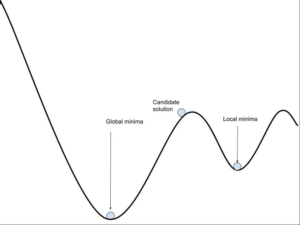
It is not a simple bowl shape with a single best set of weights that we are guaranteed to find. Instead, there is a landscape of peaks and valleys with many good and many misleadingly good sets of parameters that we may discover.
Solving this optimization is challenging, not least because the error surface contains many local optima, flat spots, and cliffs.
An iterative process must be used to navigate the non-convex error surface of the model. A naive algorithm that navigates the error is likely to become misled, lost, and ultimately stuck, resulting in a poorly performing model.
Navigating the Non-Convex Error Surface
Neural network models can be thought to learn by navigating a non-convex error surface.
A model with a specific set of weights can be evaluated on the training dataset and the average error over all training datasets can be thought of as the error of the model. A change to the model weights will result in a change to the model error. Therefore, we seek a set of weights that result in a model with a small error.
This involves repeating the steps of evaluating the model and updating the model parameters in order to step down the error surface. This process is repeated until a set of parameters is found that is good enough or the search process gets stuck.
This is a search or an optimization process and we refer to optimization algorithms that operate in this way as gradient optimization algorithms, as they naively follow along the error gradient. They are computationally expensive, slow, and their empirical behavior means that using them in practice is more art than science.
The algorithm that is most commonly used to navigate the error surface is called stochastic gradient descent, or SGD for short.
Nearly all of deep learning is powered by one very important algorithm: stochastic gradient descent or SGD.
— Page 151, Deep Learning, 2016.
Other global optimization algorithms designed for non-convex optimization problems could be used, such as a genetic algorithm, but stochastic gradient descent is more efficient as it uses the gradient information specifically to update the model weights via an algorithm called backpropagation.
[Backpropagation] describes a method to calculate the derivatives of the network training error with respect to the weights by a clever application of the derivative chain-rule.
— Page 49, Neural Smithing: Supervised Learning in Feedforward Artificial Neural Networks, 1999.
Backpropagation refers to a technique from calculus to calculate the derivative (e.g. the slope or the gradient) of the model error for specific model parameters, allowing model weights to be updated to move down the gradient. As such, the algorithm used to train neural networks is also often referred to as simply backpropagation.
Actually, back-propagation refers only to the method for computing the gradient, while another algorithm, such as stochastic gradient descent, is used to perform learning using this gradient.
— Page 204, Deep Learning, 2016.
Stochastic gradient descent can be used to find the parameters for other machine learning algorithms, such as linear regression, and it is used when working with very large datasets, although if there are sufficient resources, then convex-based optimization algorithms are significantly more efficient.
Components of the Learning Algorithm
Training a deep learning neural network model using stochastic gradient descent with backpropagation involves choosing a number of components and hyperparameters. In this section, we’ll take a look at each in turn.
An error function must be chosen, often called the objective function, cost function, or the loss function. Typically, a specific probabilistic framework for inference is chosen called Maximum Likelihood. Under this framework, the commonly chosen loss functions are cross entropy for classification problems and mean squared error for regression problems.
- Loss Function. The function used to estimate the performance of a model with a specific set of weights on examples from the training dataset.
The search or optimization process requires a starting point from which to begin model updates. The starting point is defined by the initial model parameters or weights. Because the error surface is non-convex, the optimization algorithm is sensitive to the initial starting point. As such, small random values are chosen as the initial model weights, although different techniques can be used to select the scale and distribution of these values. These techniques are referred to as “weight initialization” methods.
- Weight Initialization. The procedure by which the initial small random values are assigned to model weights at the beginning of the training process.
When updating the model, a number of examples from the training dataset must be used to calculate the model error, often referred to simply as “loss.” All examples in the training dataset may be used, which may be appropriate for smaller datasets. Alternately, a single example may be used which may be appropriate for problems where examples are streamed or where the data changes often. A hybrid approach may be used where the number of examples from the training dataset may be chosen and used to estimate the error gradient. The choice of the number of examples is referred to as the batch size.
- Batch Size. The number of examples used to estimate the error gradient before updating the model parameters.
Once an error gradient has been estimated, the derivative of the error can be calculated and used to update each parameter. There may be statistical noise in the training dataset and in the estimate of the error gradient. Also, the depth of the model (number of layers) and the fact that model parameters are updated separately means that it is hard to calculate exactly how much to change each model parameter to best move down the whole model down the error gradient.
Instead, a small portion of the update to the weights is performed each iteration. A hyperparameter called the “learning rate” controls how much to update model weights and, in turn, controls how fast a model learns on the training dataset.
- Learning Rate: The amount that each model parameter is updated per cycle of the learning algorithm.
The training process must be repeated many times until a good or good enough set of model parameters is discovered. The total number of iterations of the process is bounded by the number of complete passes through the training dataset after which the training process is terminated. This is referred to as the number of training “epochs.”
- Epochs. The number of complete passes through the training dataset before the training process is terminated.
There are many extensions to the learning algorithm, although these five hyperparameters generally control the learning algorithm for deep learning neural networks.
Further Reading
This section provides more resources on the topic if you are looking to go deeper.
- Deep Learning, 2016.
- Neural Smithing: Supervised Learning in Feedforward Artificial Neural Networks, 1999.
- Neural Networks for Pattern Recognition, 1995.
Summary
In this post, you discovered the challenge of finding model parameters for deep learning neural networks.
Specifically, you learned:
- Neural networks learn a mapping function from inputs to outputs that can be summarized as solving the problem of function approximation.
- Unlike other machine learning algorithms, the parameters of a neural network must be found by solving a non-convex optimization problem with many good solutions and many misleadingly good solutions.
- The stochastic gradient descent algorithm is used to solve the optimization problem where model parameters are updated each iteration using the backpropagation algorithm.
Do you have any questions?
Ask your questions in the comments below and I will do my best to answer.


One question:
It is written
“Stochastic gradient descent can be used to find the parameters for other machine learning algorithms, such as linear regression, and it is used when working with very large datasets, although if there are sufficient resources, then convex-based optimization algorithms are significantly more efficient.”
What does that mean ” if there are sufficient resources, then convex-based optimization algorithms are significantly more efficient”.
Does that mean that given the same data-set, the objective function is non convex if one use stochastic gradient descent (or mini-batch gradient descent), but the objective function becomes convex if one use ‘full’ batch gradient descent [assuming enough computation res sources]
I mean if all of the data can fit in RAM and that the solver can run in a reasonable time, and that the data is suitably prepared for the expectations of the convex optimization algorithm.
SGD can efficiently approximate the same convex optimization problem.
Thanks Jason.
that article is useful [for some people reading this post who have same kind of interrogation as me]
https://www.oreilly.com/ideas/the-hard-thing-about-deep-learning
Thanks for sharing.
Hi sir,
what do we mean by non-convex optimization problem? since i am a little bit confused.
thank you.
Sorry, it means a much harder problem, e.g. a problem where the error surface is not a smooth bowl for the algorithm to navigate.
adnane… pick any 2 lo points in set and connect these two points by stright line then full line need to be psrt of sane set. this should be true for any teo points in the same set.. if it so then it is called as convex set
Hi sir,
history = model.fit(X, y, batch_size=10, epochs=100) this code fit model . i know. but batch size and epochs is back propagation or not sir
Yes, neural networks in Keras are fit using backpropagation.
Why isn’t ” batch_size = 1 ” a good idea ?
Slow. Noisy estimate of the gradient.
Points in : “Components of the Learning Algorithm” has definitions jumbled .
Please fix the paragraphs for : Batch Size, Learning Rate, Epoch , Loss Function and
Weight Initialization..
What is jumbled exactly?
What is the difference between initialization of a neural network and training a neural network? without using any math formulas.
Initialization is the starting point for the optimization.
Training is the actual optimization process itself.