Model ensembles can achieve lower generalization error than single models but are challenging to develop with deep learning neural networks given the computational cost of training each single model.
An alternative is to train multiple model snapshots during a single training run and combine their predictions to make an ensemble prediction. A limitation of this approach is that the saved models will be similar, resulting in similar predictions and predictions errors and not offering much benefit from combining their predictions.
Effective ensembles require a diverse set of skillful ensemble members that have differing distributions of prediction errors. One approach to promoting a diversity of models saved during a single training run is to use an aggressive learning rate schedule that forces large changes in the model weights and, in turn, the nature of the model saved at each snapshot.
In this tutorial, you will discover how to develop snapshot ensembles of models saved using an aggressive learning rate schedule over a single training run.
After completing this tutorial, you will know:
Snapshot ensembles combine the predictions from multiple models saved during a single training run.
Diversity in model snapshots can be achieved through the use of aggressively cycling the learning rate used during a single training run.
How to save model snapshots during a single run and load snapshot models to make ensemble predictions.
Kick-start your project with my new book Better Deep Learning, including step-by-step tutorials and the Python source code files for all examples.
Let’s get started.
Updated Oct/2019: Updated for Keras 2.3 and TensorFlow 2.0.
Update Jan/2020: Updated for changes in scikit-learn v0.22 API.
How to Develop a Snapshot Ensemble Deep Learning Neural Network in Python With Keras Photo by Jason Jacobs, some rights reserved.
Tutorial Overview
This tutorial is divided into five parts; they are:
Snapshot Ensembles
Multi-Class Classification Problem
Multilayer Perceptron Model
Cosine Annealing Learning Rate
MLP Snapshot Ensemble
Snapshot Ensembles
A problem with ensemble learning with deep learning methods is the large computational cost of training multiple models.
This is because of the use of very deep models and very large datasets that can result in model training times that may extend to days, weeks, or even months.
Despite its obvious advantages, the use of ensembling for deep networks is not nearly as widespread as it is for other algorithms. One likely reason for this lack of adaptation may be the cost of learning multiple neural networks. Training deep networks can last for weeks, even on high performance hardware with GPU acceleration.
One approach to ensemble learning for deep learning neural networks is to collect multiple models from a single training run. This addresses the computational cost of training multiple deep learning models as models can be selected and saved during training, then used to make an ensemble prediction.
A key benefit of ensemble learning is in improved performance compared to the predictions from single models. This can be achieved through the selection of members that have good skill, but in different ways, providing a diverse set of predictions to be combined. A limitation of collecting multiple models during a single training run is that the models may be good, but too similar.
This can be addressed by changing the learning algorithm for the deep neural network to force the exploration of different network weights during a single training run that will result, in turn, with models that have differing performance. One way that this can be achieved is by aggressively changing the learning rate used during training.
An approach to systematically and aggressively changing the learning rate during training to result in very different network weights is referred to as “Stochastic Gradient Descent with Warm Restarts” or SGDR for short, described by Ilya Loshchilov and Frank Hutter in their 2017 paper “SGDR: Stochastic Gradient Descent with Warm Restarts.”
Their approach involves systematically changing the learning rate over training epochs, called cosine annealing. This approach requires the specification of two hyperparameters: the initial learning rate and the total number of training epochs.
The “cosine annealing” method has the effect of starting with a large learning rate that is relatively rapidly decreased to a minimum value before being dramatically increased again. The model weights are subjected to the dramatic changes during training, having the effect of using “good weights” as the starting point for the subsequent learning rate cycle, but allowing the learning algorithm to converge to a different solution.
The resetting of the learning rate acts like a simulated restart of the learning process and the re-use of good weights as the starting point of the restart is referred to as a “warm restart,” in contrast to a “cold restart” where a new set of small random numbers may be used as a starting point.
The “good weights” at the bottom of each cycle can be saved to file, providing a snapshot of the model. These snapshots can be collected together at the end of the run and used in a model averaging ensemble. The saving and use of these models during an aggressive learning rate schedule is referred to as a “Snapshot Ensemble” and was described by Gao Huang, et al. in their 2017 paper titled “Snapshot Ensembles: Train 1, get M for free” and subsequently also used in an updated version of the Loshchilov and Hutter paper.
… we let SGD converge M times to local minima along its optimization path. Each time the model converges, we save the weights and add the corresponding network to our ensemble. We then restart the optimization with a large learning rate to escape the current local minimum.
The ensemble of models is created during the course of training a single model, therefore, the authors claim that the ensemble forecast is provided at no additional cost.
[the approach allows] learning an ensemble of multiple neural networks without incurring any additional training costs.
Although a cosine annealing schedule is used for the learning rate, other aggressive learning rate schedules could be used, such as the simpler cyclical learning rate schedule described by Leslie Smith in the 2017 paper titled “Cyclical Learning Rates for Training Neural Networks.”
Now that we are familiar with the snapshot ensemble technique, we can look at how to implement it in Python with Keras.
Want Better Results with Deep Learning?
Take my free 7-day email crash course now (with sample code).
Click to sign-up and also get a free PDF Ebook version of the course.
Multi-Class Classification Problem
We will use a small multi-class classification problem as the basis to demonstrate the snapshot ensemble.
The scikit-learn class provides the make_blobs() function that can be used to create a multi-class classification problem with the prescribed number of samples, input variables, classes, and variance of samples within a class.
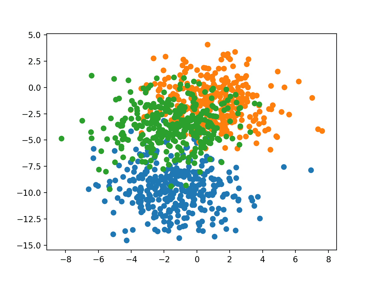
The problem has two input variables (to represent the x and y coordinates of the points) and a standard deviation of 2.0 for points within each group. We will use the same random state (seed for the pseudorandom number generator) to ensure that we always get the same data points.
The result is the input and output elements of a dataset that we can model.
In order to get a feeling for the complexity of the problem, we can plot each point on a two-dimensional scatter plot and color each point by class value.
Running the example creates a scatter plot of the entire dataset. We can see that the standard deviation of 2.0 means that the classes are not linearly separable (separable by a line) causing many ambiguous points.
This is desirable as it means that the problem is non-trivial and will allow a neural network model to find many different “good enough” candidate solutions resulting in a high variance.
Scatter Plot of Blobs Dataset With Three Classes and Points Colored by Class Value
Multilayer Perceptron Model
Before we define a model, we need to contrive a problem that is appropriate for the ensemble.
In our problem, the training dataset is relatively small. Specifically, there is a 10:1 ratio of examples in the training dataset to the holdout dataset. This mimics a situation where we may have a vast number of unlabeled examples and a small number of labeled examples with which to train a model.
We will create 1,100 data points from the blobs problem. The model will be trained on the first 100 points and the remaining 1,000 will be held back in a test dataset, unavailable to the model.
The problem is a multi-class classification problem, and we will model it using a softmax activation function on the output layer. This means that the model will predict a vector with three elements with the probability that the sample belongs to each of the three classes. Therefore, we must one hot encode the class values before we split the rows into the train and test datasets. We can do this using the Keras to_categorical() function.
The model will expect samples with two input variables. The model then has a single hidden layer with 25 nodes and a rectified linear activation function, then an output layer with three nodes to predict the probability of each of the three classes and a softmax activation function.
Because the problem is multi-class, we will use the categorical cross entropy loss function to optimize the model and stochastic gradient descent with a small learning rate and momentum.
Running the example prints the performance of the final model on the train and test datasets.
Note: Your results may vary given the stochastic nature of the algorithm or evaluation procedure, or differences in numerical precision. Consider running the example a few times and compare the average outcome.
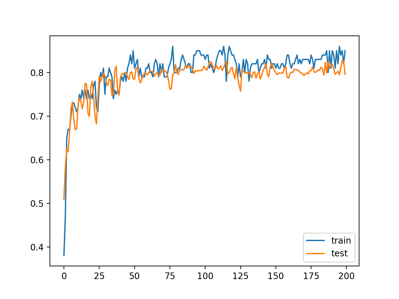
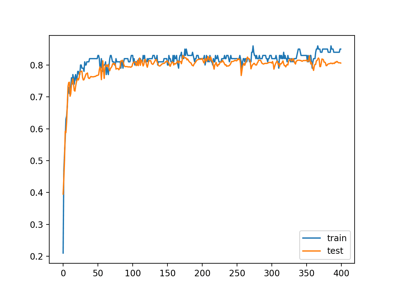
In this case, we can see that the model achieved about 84% accuracy on the training dataset, which we know is optimistic, and about 79% on the test dataset, which we would expect to be more realistic.
1
Train: 0.840, Test: 0.796
A line plot is also created showing the learning curves for the model accuracy on the train and test sets over each training epoch.
We can see that training accuracy is more optimistic over most of the run as we also noted with the final scores.
Line Plot Learning Curves of Model Accuracy on Train and Test Dataset over Each Training Epoch
Next, we can look at how to implement an aggressive learning rate schedule.
Cosine Annealing Learning Rate
An effective snapshot ensemble requires training a neural network with an aggressive learning rate schedule.
The cosine annealing schedule is an example of an aggressive learning rate schedule where learning rate starts high and is dropped relatively rapidly to a minimum value near zero before being increased again to the maximum.
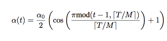
We can implement the schedule as described in the 2017 paper “Snapshot Ensembles: Train 1, get M for free.” The equation requires the total training epochs, maximum learning rate, and number of cycles as arguments as well as the current epoch number. The function then returns the learning rate for the given epoch.
Equation for the Cosine Annealing Learning Rate Schedule Where a(t) is the learning rate at epoch t, a0 is the maximum learning rate, T is the total epochs, M is the number of cycles, mod is the modulo operation, and square brackets indicate a floor operation. Taken from “Snapshot Ensembles: Train 1, get M for free”.
The function cosine_annealing() below implements the equation.
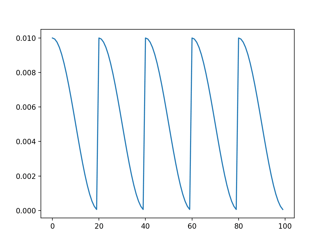
We can test this implementation by plotting the learning rate over 100 epochs with five cycles (e.g. 20 epochs long) and a maximum learning rate of 0.01. The complete example is listed below.
1
2
3
4
5
6
7
8
9
10
11
12
13
14
15
16
17
18
19
20
# example of a cosine annealing learning rate schedule
Running the example creates a line plot of the learning rate schedule over 100 epochs.
We can see that the learning rate starts at the maximum value at epoch 0 and decreases rapidly to epoch 19, before being reset at epoch 20, the start of the next cycle. The cycle is repeated five times as specified in the argument.
Line Plot of Cosine Annealing Learning Rate Schedule
We can implement this schedule as a custom callback in Keras. This allows the parameters of the schedule to be specified and for the learning rate to be logged so we can ensure it had the desired effect.
A custom callback can be defined as a Python class that extends the Keras Callback class.
In the class constructor, we can take the required configuration as arguments and save them for use, specifically the total number of training epochs, the number of cycles for the learning rate schedule, and the maximum learning rate.
We can use our cosine_annealing() defined above to calculate the learning rate for a given training epoch.
The Callback class allows an on_epoch_begin() function to be overridden that will be called prior to each training epoch. We can override this function to calculate the learning rate for the current epoch and set it in the optimizer. We can also keep track of the learning rate in an internal list.
We can create an instance of the callback and set the arguments. We will train the model for 400 epochs and set the number of cycles to be 50 epochs long, or 500 / 50, a suggestion made and configuration used throughout the snapshot ensembles paper.
We lower the learning rate at a very fast pace, encouraging the model to converge towards its first local minimum after as few as 50 epochs.
The paper also suggests that the learning rate can be set each sample or each mini-batch instead of prior to each epoch to give more nuance to the updates, but we will leave this as a future exercise.
… we update the learning rate at each iteration rather than at every epoch. This improves the convergence of short cycles, even when a large initial learning rate is used.
Once the callback is instantiated and configured, we can specify it as part of the list of callbacks to the call to the fit() function to train the model.
At the end of the run, we can confirm that the learning rate schedule was performed by plotting the contents of the lrates list.
1
2
3
# plot learning rate
pyplot.plot(ca.lrates)
pyplot.show()
Tying these elements together, the complete example of training an MLP on the blobs problem with a cosine annealing learning rate schedule is listed below.
1
2
3
4
5
6
7
8
9
10
11
12
13
14
15
16
17
18
19
20
21
22
23
24
25
26
27
28
29
30
31
32
33
34
35
36
37
38
39
40
41
42
43
44
45
46
47
48
49
50
51
52
53
54
55
56
57
58
59
60
61
62
63
64
65
66
67
68
69
# mlp with cosine annealing learning rate schedule on blobs problem
Running the example first reports the accuracy of the model on the training and test sets.
Note: Your results may vary given the stochastic nature of the algorithm or evaluation procedure, or differences in numerical precision. Consider running the example a few times and compare the average outcome.
In this case, we do not see much difference in the performance of the final model as compared to the previous section.
1
Train: 0.850, Test: 0.806
A line plot of the learning rate schedule is created, showing eight cycles of 50 epochs each.
Cosine Annealing Learning Rate Schedule While Fitting an MLP on the Blobs Problem
Finally, a line plot of model accuracy on the train and test sets is created over each training epoch.
We can see that although the learning rate was changed dramatically, there was not a dramatic effect on model accuracy, likely because the chosen classification problem is not very difficult.
Line Plot of Train and Test Set Accuracy on the Blobs Dataset With a Cosine Annealing Learning Rate Schedule
Now that we know how to implement the cosine annealing learning schedule, we can use it to prepare a snapshot ensemble.
MLP Snapshot Ensemble
We can develop a snapshot ensemble in two parts.
The first part involves creating a custom callback to save the model at the bottom of each learning rate schedule. The second part involves loading the saved models and using them to make an ensemble prediction.
Save Snapshot Models During Training
The CosineAnnealingLearningRateSchedule can be updated to override the on_epoch_end() function called at the end of each training epoch. In this function, we can check if the current epoch that just ended was the end of a cycle. If so, we can save the model to file.
Below is the updated callback, named the SnapshotEnsemble class.
A debug message is printed each time a model is saved as confirmation that models are being saved at the right time. For example, with 50-epoch long cycles, we would expect a model to be saved on epoch 49, 99, etc. and the learning rate reset at epoch 50, 100, etc.
1
2
3
4
5
6
7
8
9
10
11
12
13
14
15
16
17
18
19
20
21
22
23
24
25
26
27
28
29
30
31
32
33
# snapshot ensemble with custom learning rate schedule
Running the example reports that 10 models were saved for the 10-ends of the cosine annealing learning rate schedule.
1
2
3
4
5
6
7
8
9
10
>saved snapshot snapshot_model_1.h5, epoch 49
>saved snapshot snapshot_model_2.h5, epoch 99
>saved snapshot snapshot_model_3.h5, epoch 149
>saved snapshot snapshot_model_4.h5, epoch 199
>saved snapshot snapshot_model_5.h5, epoch 249
>saved snapshot snapshot_model_6.h5, epoch 299
>saved snapshot snapshot_model_7.h5, epoch 349
>saved snapshot snapshot_model_8.h5, epoch 399
>saved snapshot snapshot_model_9.h5, epoch 449
>saved snapshot snapshot_model_10.h5, epoch 499
Load Models and Make Ensemble Prediction
Once the snapshot models have been saved to file, they can be loaded and used to make an ensemble prediction.
The first step is to load the models into memory. For large models, this could be done one model at a time, make a prediction, and move on to the next model before combining predictions. In this case, the models are relatively small and we can load all 10 from file as a list.
1
2
3
4
5
6
7
8
9
10
11
12
# load models from file
def load_all_models(n_models):
all_models=list()
foriinrange(n_models):
# define filename for this ensemble
filename='snapshot_model_'+str(i+1)+'.h5'
# load model from file
model=load_model(filename)
# add to list of members
all_models.append(model)
print('>loaded %s'%filename)
returnall_models
We would expect that models saved towards the end of the run may have better performance than models saved earlier in the run. As such, we can reverse the list of loaded models so that the older models are first.
1
2
# reverse loaded models so we build the ensemble with the last models first
members=list(reversed(members))
We don’t know how many snapshots are required to make a good prediction for this problem. We can explore the effect of the number of ensemble members on test set accuracy by creating ensembles of increasing size starting with the final model at epoch 499, then adding the model saved at epoch 449, and so on until all 10 models are included.
First, we require a function to make a prediction given a list of models. Given that each model predicts the probabilities of each of the output classes, we can sum the predicted probabilities across the models and select the class with the most support via the argmax() function. The ensemble_predictions() function below implements this functionality.
1
2
3
4
5
6
7
8
9
10
# make an ensemble prediction for multi-class classification
def ensemble_predictions(members,testX):
# make predictions
yhats=[model.predict(testX)formodel inmembers]
yhats=array(yhats)
# sum across ensemble members
summed=numpy.sum(yhats,axis=0)
# argmax across classes
result=argmax(summed,axis=1)
returnresult
We can then evaluate an ensemble of a given size by selecting the first n members from the list of models, making a prediction by calling the ensemble_predictions() function, and then calculating and returning the accuracy of the prediction. The evaluate_n_members() function below implements this behavior.
1
2
3
4
5
6
7
8
# evaluate a specific number of members in an ensemble
The performance of each ensemble can also be contrasted with the performance of each standalone model and the average performance of all standalone models.
1
2
3
4
5
6
7
8
9
10
11
12
13
14
# evaluate different numbers of ensembles on hold out set
Finally, we can plot the performance of each individual snapshot model (blue dots) compared to the performance of an ensemble that includes all models up to and including each individual model (orange line).
Running the example first loads all 10 models into memory.
1
2
3
4
5
6
7
8
9
10
11
>loaded snapshot_model_1.h5
>loaded snapshot_model_2.h5
>loaded snapshot_model_3.h5
>loaded snapshot_model_4.h5
>loaded snapshot_model_5.h5
>loaded snapshot_model_6.h5
>loaded snapshot_model_7.h5
>loaded snapshot_model_8.h5
>loaded snapshot_model_9.h5
>loaded snapshot_model_10.h5
Loaded 10 models
Next, each snapshot model is evaluated on the test dataset and the accuracy is reported. This is contrasted with the accuracy of a snapshot ensemble that includes all snapshot models working backward from the end of the run including the single model.
The results show that as we work backward from the end of the run, the performance of the snapshot models gets worse, as we might expect.
Note: Your results may vary given the stochastic nature of the algorithm or evaluation procedure, or differences in numerical precision. Consider running the example a few times and compare the average outcome.
Combining snapshot models into an ensemble shows that performance increases up to and including the last 3-to-5 models, reaching about 82%. This can be compared to the average performance of a snapshot model of about 80% test set accuracy.
1
2
3
4
5
6
7
8
9
10
11
> 1: single=0.813, ensemble=0.813
> 2: single=0.814, ensemble=0.813
> 3: single=0.822, ensemble=0.822
> 4: single=0.810, ensemble=0.820
> 5: single=0.813, ensemble=0.818
> 6: single=0.811, ensemble=0.815
> 7: single=0.807, ensemble=0.813
> 8: single=0.805, ensemble=0.813
> 9: single=0.805, ensemble=0.813
> 10: single=0.790, ensemble=0.813
Accuracy 0.809 (0.008)
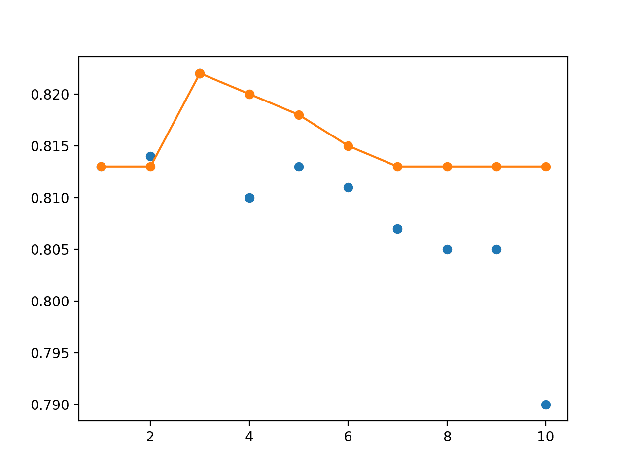
Finally, a line plot is created plotting the same test set accuracy scores.
We can set the performance of each individual snapshot model as a blue dot and the snapshot ensemble of increasing size (number of members) from 1 to 10 members as an orange line.
At least on this run, we can see that the snapshot ensemble quickly out-performs the final model at 82.2% with 3 members and all other saved models before performance degrades back down to about the same as the final model at 81.3%.
Line Plot of Single Snapshot Models (blue dots) vs Snapshot Ensembles of Varied Sized (orange line)
Extensions
This section lists some ideas for extending the tutorial that you may wish to explore.
Vary Cycle Length. Update the example to use a shorter or longer cycle length and compare results.
Vary Maximum Learning Rate. Update the example to use a larger or smaller maximum learning rate and compare results.
Update Learning Rate Per Batch. Update the example to calculate the learning rate per-batch instead of per-epoch.
Repeated Evaluation. Update the example to repeat the evaluation of the model to confirm that the approach indeed leads to an improved performance over the final model on the blobs problem.
Cyclic Learning Rate. Update the example to use a cyclic learning rate schedule and compare results.
If you explore any of these extensions, I’d love to know.
Further Reading
This section provides more resources on the topic if you are looking to go deeper.
In this tutorial, you discovered how to develop snapshot ensembles of models saved using an aggressive learning rate schedule over a single training run.
Specifically, you learned:
Snapshot ensembles combine the predictions from multiple models saved during a single training run.
Diversity in model snapshots can be achieved through the use of aggressively cycling the learning rate used during a single training run.
How to save model snapshots during a single run and load snapshot models to make ensemble predictions.
Do you have any questions?
Ask your questions in the comments below and I will do my best to answer.
Thank you again for this great article. However, I have some confusion and question please.
1) yhats = [model.predict(testX) for model in members]
Q. model.predict_proba(testX) as we are predicting the probabilities?
2) now that we identify that ensemble shows that performance increases up to and including the last 3-to-5 models.
Q. how can we make a final prediction on a holdout data for submission (in case of competition) using the ensemble model?
Is it okay to collect multiple models based on test set not validation set
during the evaluation process of the model?
If this is the information leakage from the test data to the model,
we’d have to use train set as validation set and
would it possibly be better to use cross validation for better performance?
Thanks sir for this great tutorial, I am following this tutorial to apply snapshot ensemble on Arabic words image to recognize but the results of last snapshots always less than last individual snapshot method
”
the number of snapshots in use 4
******************************
4561 correct / 5029 total
The total loss of model no 0 : 0.351080983877182 and accuracy = 90.69397494531717 %
******************************
4589 correct / 5029 total
The total loss of model no 1 : 0.34880080819129944 and accuracy = 91.25074567508452 %
******************************
4613 correct / 5029 total
The total loss of model no 2 : 0.35147425532341003 and accuracy = 91.7279777291708 %
******************************
4613 correct / 5029 total
The total loss of model no 3 : 0.3585134446620941 and accuracy = 91.7279777291708 %
******************************
Acc of 4 snapshots = 91.50924637104792 %
No of correct 4602/5029total
”
is this could happens ?
This is the link of my test ensemble function https://colab.research.google.com/drive/1Qzbh_sjUtd12KPUVISvZzkCyGdW4Hd2a#scrollTo=TPxNw2SeIMBo
Thank you very much, BTW I see these days you posted a very nice tutorial about Pytorch so I suggest you to use both in your new examples if it is possible
Hi Jason,
I would like to implement sth different for my data. My aim is to apply adaptive dropout rate for differen epoch intervals. My custom callback inspired by yours is as follows:
class MyDropCallback(Callback):
def __init__(self,dropping_rate):
self.dropping_rate=dropping_rate
As you see at the bottom line of the code above, i am not sure what to write there. If it was a learning rate schedule, it would be written self.model.optimizer.lr. What do you suggest for this issue?
Thanks from now on
Hello Dr. Brownlee. Thanks for your nice tutorial.
I faced to an error while implementing this technique.
I have 7 different CNN models that are saved on disk. After loading them, I use predict_generator to apply prediction for each model.
# make an ensemble prediction for multi-class classification
def ensemble_predictions(members):
# make predictions
yhats = [model.model.predict_generator(test_generator, evaluate_generator_steps, max_queue_size = 2, workers = 1) for model in members]
yhats = array(yhats)
# sum across ensemble members
summed = numpy.sum(yhats, axis=0)
# argmax across classes
result = argmax(summed, axis=1)
return result
But I got the following error :
—————————————————————————
InvalidArgumentError Traceback (most recent call last)
in ()
8 shuffle=False)
9
—> 10 probabilities = members[0].predict_generator(test_generator, evaluate_generator_steps, max_queue_size = 2, workers = 1)
10 frames
/usr/local/lib/python3.6/dist-packages/tensorflow/python/eager/execute.py in quick_execute(op_name, num_outputs, inputs, attrs, ctx, name)
58 ctx.ensure_initialized()
59 tensors = pywrap_tfe.TFE_Py_Execute(ctx._handle, device_name, op_name,
—> 60 inputs, attrs, num_outputs)
61 except core._NotOkStatusException as e:
62 if name is not None:
InvalidArgumentError: Input to reshape is a tensor with 64000 values, but the requested shape requires a multiple of 4608
[[node sequential_1/flatten_1/Reshape (defined at :18) ]] [Op:__inference_predict_function_105280]
InvalidArgumentError Traceback (most recent call last)
in ()
2 for i in range(1, len(members)+1):
3 # evaluate model with i members
—-> 4 ensemble_score = evaluate_n_members(members, i)
5 # evaluate the i’th model standalone
6 _, single_score = members[i-1].evaluate_generator(test_generator, evaluate_generator_steps, max_queue_size = 2, workers = 1)
12 frames
/usr/local/lib/python3.6/dist-packages/tensorflow/python/eager/execute.py in quick_execute(op_name, num_outputs, inputs, attrs, ctx, name)
58 ctx.ensure_initialized()
59 tensors = pywrap_tfe.TFE_Py_Execute(ctx._handle, device_name, op_name,
—> 60 inputs, attrs, num_outputs)
61 except core._NotOkStatusException as e:
62 if name is not None:
InvalidArgumentError: Input to reshape is a tensor with 64000 values, but the requested shape requires a multiple of 4608
[[node sequential_1/flatten_1/Reshape (defined at :18) ]] [Op:__inference_predict_function_105280]
Dr. Brownlee, I have a question regarding argmax function. Should I use argmax for binary classification?
Especially, in “ensemble_predictions” function, you used argmax. When I apply argmax, all predictions change to zero.
Thanks sir for your time and patience. Could you please explain briefly regarding reason and advantage of using of sum function before argmax in your code?


")


Hello Jason,
Great post! I am quite interested in ML within audio processing /recognition field.
Any chance you could kindly help out and suggest how to practically build phoneme classifier python using TIMIT dataset? http://academictorrents.com/details/34e2b78745138186976cbc27939b1b34d18bd5b3
There are papers on the subject (eg A. Graves). However, it is difficult to get started based only on that.
I would lie to build a phoneme classifier (based on cnn or lstm) with apox. 70% accuracy.
Any blog post dedicated with practical suggestions would be highly appreciated!
thanks and regards
I would love to cover this topic in the future, thanks for the suggestion.
Hi Jason,
Thank you again for this great article. However, I have some confusion and question please.
1) yhats = [model.predict(testX) for model in members]
Q. model.predict_proba(testX) as we are predicting the probabilities?
2) now that we identify that ensemble shows that performance increases up to and including the last 3-to-5 models.
Q. how can we make a final prediction on a holdout data for submission (in case of competition) using the ensemble model?
Hope my question is clear enough.
Thanks again Jason.
Dennis
No need, we get softmax probabilities from predict().
Call ensemble_predictions() to make a prediction on new data with the members.
Thanks Jason for clearing up some confusion. You made my day!
I’m glad it helped.
Cheers mate for this brilliant post!
Is it okay to collect multiple models based on test set not validation set
during the evaluation process of the model?
If this is the information leakage from the test data to the model,
we’d have to use train set as validation set and
would it possibly be better to use cross validation for better performance?
Thank you so much.
Ideally, you would use a validation dataset. I use the test set to keep the example simple.
Thanks sir for this great tutorial, I am following this tutorial to apply snapshot ensemble on Arabic words image to recognize but the results of last snapshots always less than last individual snapshot method
”
the number of snapshots in use 4
******************************
4561 correct / 5029 total
The total loss of model no 0 : 0.351080983877182 and accuracy = 90.69397494531717 %
******************************
4589 correct / 5029 total
The total loss of model no 1 : 0.34880080819129944 and accuracy = 91.25074567508452 %
******************************
4613 correct / 5029 total
The total loss of model no 2 : 0.35147425532341003 and accuracy = 91.7279777291708 %
******************************
4613 correct / 5029 total
The total loss of model no 3 : 0.3585134446620941 and accuracy = 91.7279777291708 %
******************************
Acc of 4 snapshots = 91.50924637104792 %
No of correct 4602/5029total
”
is this could happens ?
This is the link of my test ensemble function
https://colab.research.google.com/drive/1Qzbh_sjUtd12KPUVISvZzkCyGdW4Hd2a#scrollTo=TPxNw2SeIMBo
Well done on your progress.
Sorry, I don’t have the capacity to review your code. I explain more here:
https://machinelearningmastery.com/faq/single-faq/can-you-read-review-or-debug-my-code
Thank you very much,
could you please let me know why you used 100 data points fro training and left 1000 data points for testing?
Best regards
Completely arbitrary. To make the problem more challenging for the model and make the example interesting.
Thank you very much, BTW I see these days you posted a very nice tutorial about Pytorch so I suggest you to use both in your new examples if it is possible
Thank you
Thanks for the suggestion.
I intend to stick with Keras for now.
Hi Jason,
I would like to implement sth different for my data. My aim is to apply adaptive dropout rate for differen epoch intervals. My custom callback inspired by yours is as follows:
class MyDropCallback(Callback):
def __init__(self,dropping_rate):
self.dropping_rate=dropping_rate
def updating_mydroprate(self,epoch,dropping_rate):
if epoch==35:
dropping_rate=0.65
elif epoch==60:
dropping_rate=0.75
elif epoch==80:
dropping_rate=0.8
def on_epoch_begin(self,epoch,logs=None):
dropping_rate=self.updating_mydroprate(epoch,self.dropping_rate)
backend.set_value(self.????????? , dropping_rate)
As you see at the bottom line of the code above, i am not sure what to write there. If it was a learning rate schedule, it would be written self.model.optimizer.lr. What do you suggest for this issue?
Thanks from now on
Sorry, I cannot help you with your custom code, perhaps post to stackoverflow?
Thx
You’re welcome.
Hello Dr. Brownlee. Thanks for your nice tutorial.
I faced to an error while implementing this technique.
I have 7 different CNN models that are saved on disk. After loading them, I use predict_generator to apply prediction for each model.
The code is as follows :
img_width, img_height = 224, 224
depth = 3
number_of_test_sample = 1172
batch_size = 20
evaluate_generator_steps = int(number_of_test_sample / batch_size) + 1
class_mode = ‘binary’
test_datagen = ImageDataGenerator(rescale=1./255)
test_generator = test_datagen.flow_from_directory(
test_dir,
target_size=(img_width, img_height),
batch_size=batch_size,
class_mode=class_mode,
shuffle=False)
# make an ensemble prediction for multi-class classification
def ensemble_predictions(members):
# make predictions
yhats = [model.model.predict_generator(test_generator, evaluate_generator_steps, max_queue_size = 2, workers = 1) for model in members]
yhats = array(yhats)
# sum across ensemble members
summed = numpy.sum(yhats, axis=0)
# argmax across classes
result = argmax(summed, axis=1)
return result
But I got the following error :
—————————————————————————
InvalidArgumentError Traceback (most recent call last)
in ()
8 shuffle=False)
9
—> 10 probabilities = members[0].predict_generator(test_generator, evaluate_generator_steps, max_queue_size = 2, workers = 1)
10 frames
/usr/local/lib/python3.6/dist-packages/tensorflow/python/eager/execute.py in quick_execute(op_name, num_outputs, inputs, attrs, ctx, name)
58 ctx.ensure_initialized()
59 tensors = pywrap_tfe.TFE_Py_Execute(ctx._handle, device_name, op_name,
—> 60 inputs, attrs, num_outputs)
61 except core._NotOkStatusException as e:
62 if name is not None:
InvalidArgumentError: Input to reshape is a tensor with 64000 values, but the requested shape requires a multiple of 4608
[[node sequential_1/flatten_1/Reshape (defined at :18) ]] [Op:__inference_predict_function_105280]
Function call stack:
predict_function
Could you please help me to solve the problem?
InvalidArgumentError Traceback (most recent call last)
in ()
2 for i in range(1, len(members)+1):
3 # evaluate model with i members
—-> 4 ensemble_score = evaluate_n_members(members, i)
5 # evaluate the i’th model standalone
6 _, single_score = members[i-1].evaluate_generator(test_generator, evaluate_generator_steps, max_queue_size = 2, workers = 1)
12 frames
/usr/local/lib/python3.6/dist-packages/tensorflow/python/eager/execute.py in quick_execute(op_name, num_outputs, inputs, attrs, ctx, name)
58 ctx.ensure_initialized()
59 tensors = pywrap_tfe.TFE_Py_Execute(ctx._handle, device_name, op_name,
—> 60 inputs, attrs, num_outputs)
61 except core._NotOkStatusException as e:
62 if name is not None:
InvalidArgumentError: Input to reshape is a tensor with 64000 values, but the requested shape requires a multiple of 4608
[[node sequential_1/flatten_1/Reshape (defined at :18) ]] [Op:__inference_predict_function_105280]
Function call stack:
predict_function
I’m sorry to hear that that. I believe this will help:
https://machinelearningmastery.com/faq/single-faq/why-does-the-code-in-the-tutorial-not-work-for-me
Thanks Dr. Brownlee. I shared my question in stackoverflow. I hope I can get the answer. But do you have any suggestion the tackle the issue?
Not off hand sorry, you will need to debug your code to find the cause of the fault.
Dr. Brownlee, I have a question regarding argmax function. Should I use argmax for binary classification?
Especially, in “ensemble_predictions” function, you used argmax. When I apply argmax, all predictions change to zero.
No need to use argmax on binary classification, use round() on the predicted probability.
Thanks sir for your time and patience. Could you please explain briefly regarding reason and advantage of using of sum function before argmax in your code?
This is called soft voting, you can learn more here:
https://machinelearningmastery.com/voting-ensembles-with-python/
Getting this error every time
AttributeError: ‘SnapshotEnsemble’ object has no attribute ‘_implements_train_batch_hooks’
Sorry to hear that, this may help:
https://machinelearningmastery.com/faq/single-faq/why-does-the-code-in-the-tutorial-not-work-for-me
All the stuff that demonstrate in the post is also simply achievable with this packages
https://github.com/simon-larsson/keras-swa
# build model
model = Sequential()
model.add(Dense(50, input_dim=2, activation=’relu’))
model.add(BatchNormalization())
model.add(Dense(3, activation=’softmax’))
model.compile(loss=’categorical_crossentropy’,
optimizer=SGD(learning_rate=0.1))
epochs = 100
start_epoch = 75
# define swa callback
swa = SWA(start_epoch=start_epoch,
lr_schedule=’cyclic’,
swa_lr=0.001,
swa_lr2=0.003,
swa_freq=3,
verbose=1)
# train
model.fit(X, y, epochs=epochs, verbose=1, callbacks=[swa])
`Thanks for sharing.
Hi,
I tried the provided sample codes several times, but always single snapshots outperformed snapshot ensembles. Any reason for this
How to modify ensemble_predictions function for a binary classification problem
Hi pathirage…The following may be of interest to you:
https://www.sciencedirect.com/science/article/abs/pii/S0031320311000458
https://stackoverflow.com/questions/30919454/sklearn-how-to-make-an-ensemble-for-two-binary-classifiers