Supervised learning is challenging, although the depths of this challenge are often learned then forgotten or willfully ignored.
This must be the case, because dwelling too long on this challenge may result in a pessimistic outlook. In spite of the challenge, we continue to wield supervised learning algorithms and they perform well in practice.
Fundamental to the challenge of supervised learning, are the concerns:
How much data is needed to reasonably approximate the unknown underlying mapping function from inputs to outputs?
How much data is needed to reasonably estimate the performance of an approximate of the mapping function?
Generally, it is common knowledge that too little training data results in a poor approximation. An over-constrained model will underfit the small training dataset, whereas an under-constrained model, in turn, will likely overfit the training data, both resulting in poor performance. Too little test data will result in an optimistic and high variance estimation of model performance.
It is critical to make this “common knowledge” concrete with worked examples.
In this post, we will work through a detailed case study for developing a Multilayer Perceptron neural network on a simple two-class classification problem. You will discover that, in practice, we don’t have enough data to learn the mapping function or to evaluate models, yet supervised learning algorithms like neural networks remain remarkably effective.
How to analyze the two circles classification problem and measure the variance introduced by the neural network learning algorithm.
How changes in the size of a training dataset directly impact the quality of the mapping function approximated by neural networks.
How the changes in the size of a test dataset directly impact the quality of the estimated in the performance of a fit neural network model.
Kick-start your project with my new book Better Deep Learning, including step-by-step tutorials and the Python source code files for all examples.
Let’s get started.
Impact of Dataset Size on Deep Learning Model Skill And Performance Estimates Photo by Eneas De Troya, some rights reserved.
Tutorial Overview
This tutorial is divided into five parts; they are:
Challenge of Supervised Learning
Introduction to the Circles Problem
Neural Network Model Variance
Study Test Accuracy vs Training Set Size
Study Test Set Size vs Test Set Accuracy
Introduction to the Circles Problem
As the basis for our exploration, we will use a very simple two-class or binary classification problem.
The scikit-learn library provides the make_circles() function that can be used to create a binary classification problem with the prescribed number of samples and statistical noise.
Each example has two input variables that define the x and y coordinates of the point on a two-dimensional plane. The points are arranged in two concentric circles (they have the same center) for the two classes.
The number of points in the dataset is specified by a parameter, half of which will be drawn from each circle. Gaussian noise can be added when sampling the points via the “noise” argument that defines the standard deviation of the noise, where 0.0 indicates no noise or points drawn exactly from the circles. The seed for the pseudorandom number generator can be specified via the “random_state” argument that allows the exact same points to be sampled each time the function is called.
The example below generates 100 examples from the two circles with no noise and a value of 1 to seed the pseudorandom number generator.
Running the example generates the points and prints the shape of the input (X) and output (y) components of the samples. We can see that there are 100 examples of inputs with two features per example for the x and y coordinates and a matching 100 examples of the output variable or class value with 1 variable.
The first five examples from the dataset are shown. We can see that the x and y components of the input variables are centered on 0.0 and have the bounds [-1, 1]. We can also see that the class values are integers for either 0 or 1 and that examples are shuffled between the classes.
1
2
3
4
5
6
(100, 2) (100,)
[-0.6472136 -0.4702282] 1
[-0.34062343 -0.72386164] 1
[-0.53582679 -0.84432793] 0
[-0.5831749 -0.54763768] 1
[ 0.50993919 -0.61641059] 1
Plot Dataset
We can re-run the example and always get the same “randomly generated” points given the same pseudorandom number generator seed.
The example below generates the same points and plots the input variables of the samples using a scatter plot. We can use the scatter() matplotlib function to create the plot and pass in all rows of the X array with the first variable for the x coordinates and the second variable for the y coordinates on the plot.
1
2
3
4
5
6
7
8
# example of creating a scatter plot of the circles dataset
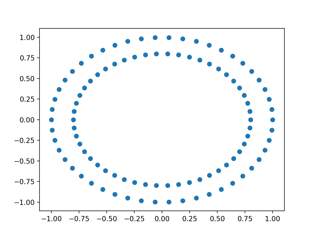
Running the example creates a scatter plot clearly showing the concentric circles of the dataset.
Scatter Plot of the Input Variables of the Circles Dataset
We can re-create the scatter plot, but instead plot all input samples for class 0 blue and all points for class 1 red.
We can select the indices of samples in the y array that have a given value using the where() NumPy function and then use those indices to select rows in the X array. The complete example is below.
1
2
3
4
5
6
7
8
9
10
11
12
13
# scatter plot of the circles dataset with points colored by class
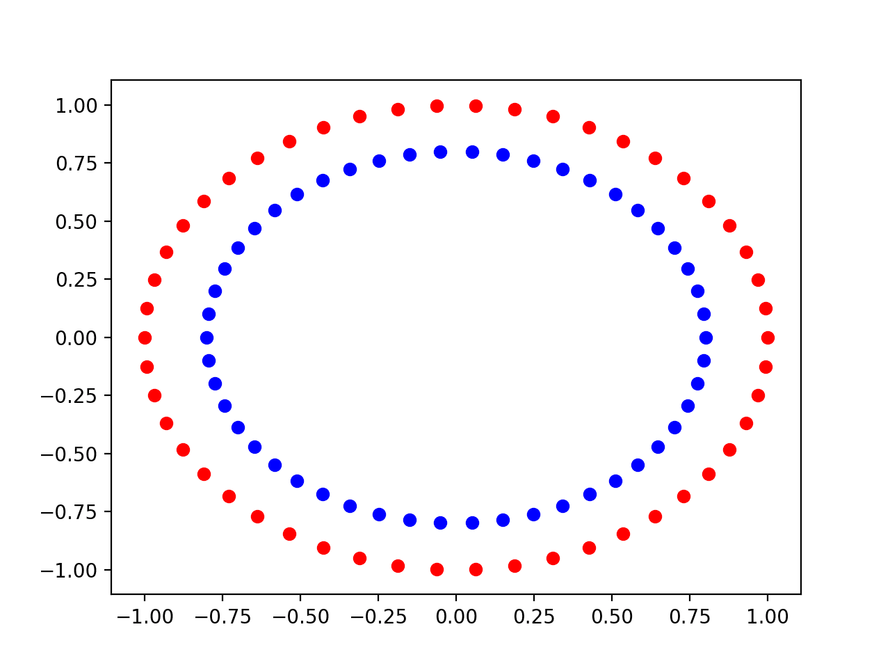
Running the example, we can see that the samples for class 0 are the inner circle in blue and samples for class belong to the outer circle in red.
Scatter Plot of the Input Variables of the Circles Dataset Colored By Class Value
Plot With Varied Noise
All real data has statistical noise. More statistical noise means that the problem is more challenging for the learning algorithm to map the input variables to the output or target variables.
The circles dataset allows us to simulate the addition of noise to the samples via the “noise” argument.
We can create a new function called scatter_plot_circles_problem() that creates a dataset with the given amount of noise and creates a scatter plot with points colored by their class value.
1
2
3
4
5
6
7
8
9
10
# create a scatter plot of the circles dataset with the given amount of noise
We can call this function multiple times with differing amounts of noise to see the effect on the complexity of the problem.
We will create four scatter plots as subplots via the subplot() matplotlib function in a 4-by-4 matrix with the noise values [0.0, 0.1, 0.2, 0.3]. The complete example is listed below.
1
2
3
4
5
6
7
8
9
10
11
12
13
14
15
16
17
18
19
20
21
22
23
# scatter plots of the circles dataset with varied amounts of noise
from sklearn.datasets import make_circles
from numpy import where
from matplotlib import pyplot
# create a scatter plot of the circles dataset with the given amount of noise
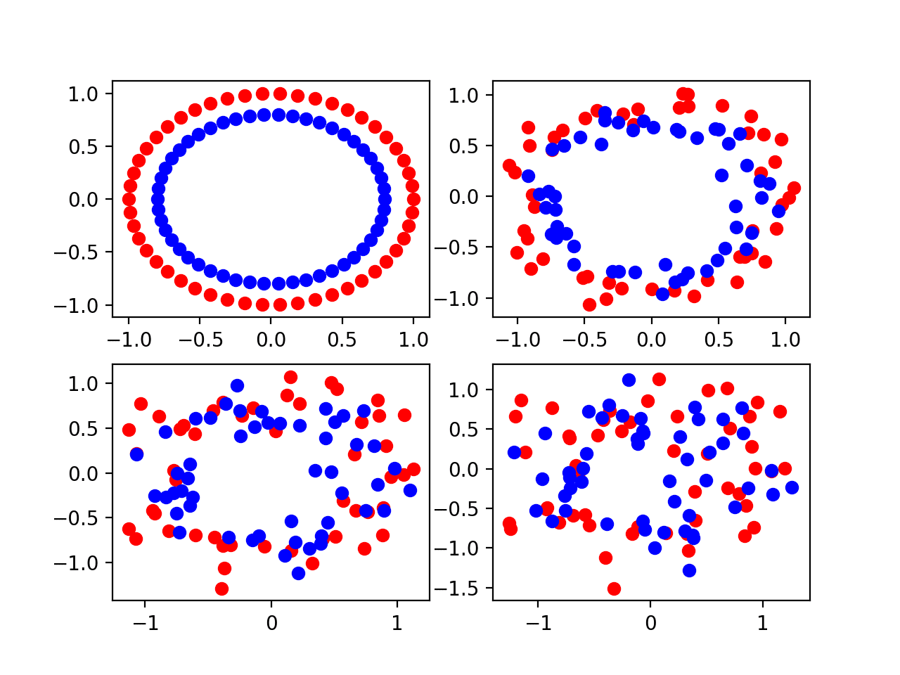
Running the example, a plot is created with four subplots, one for each of the four different noise values [0.0, 0.1, 0.2, 0.3] in the top left, top right, bottom left, and bottom right respectively.
We can see that a small amount of noise 0.1 makes the problem challenging, but still distinguishable. A noise value of 0.0 is not realistic and a dataset so perfect would not require machine learning. A noise value of 0.2 makes the problem very challenging and a value of 0.3 may the problem too challenging to learn.
Four Scatter Plots of the Circles Dataset Varied by the Amount of Statistical Noise
Plot With Varied Sample Size
We can create a similar plot of the problem with a varied number of samples.
More samples give a learning algorithm more opportunity to understand the underlying mapping of inputs to outputs, and, in turn, a better performing model.
We can update the scatter_plot_circles_problem() function to take the number of samples to generate as an argument as well as the amount of noise, and set a default for the noise of 0.1, which makes the problem noisy, but not too noisy.
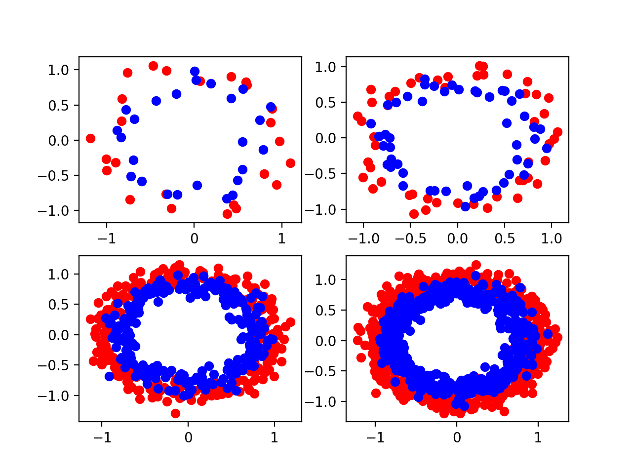
Running the example creates a plot with four subplots, one for each of the different sized samples [50, 100, 500, 1000] in the top left, top right, bottom left, and bottom right respectively.
We can see that 50 examples are probably too few and even 100 points do not look sufficient to really learn the problem. The plots suggest that 500 and 1,000 examples may be significantly easier to learn, although hide the fact that many “outlier” points result in overlaps between the two circles.
Four Scatter Plots of the Circles Dataset Varied by the Amount of Samples
Want Better Results with Deep Learning?
Take my free 7-day email crash course now (with sample code).
Click to sign-up and also get a free PDF Ebook version of the course.
Neural Network Model Variance
We can model the circles problem with a neural network.
Specifically, we can train a Multilayer Perceptron model, or MLP for short, providing input and output examples generated from the circles problem to the model. Once learned, we can evaluate how well the model has learned the problem by using it to make predictions on new examples and evaluate the accuracy.
We can develop a small MLP for the problem using the Keras deep learning library with two inputs, 25 nodes in the hidden layer, and one output. A rectified linear activation function can be used for the nodes in the hidden layer. Because the problem is a binary classification problem, the model can use the sigmoid activation function on the output layer to predict the probability of a sample belonging to class 0 or 1.
The model can be trained using an efficient version of mini-batch stochastic gradient descent called Adam, where each weight in the model has its own adaptive learning rate. The binary cross entropy loss function can be used as the basis for optimization, where smaller loss values indicate a better model fit.
We require samples generated from the circles problem to train the model and a separate test set not used to train the model that can be used estimate how well the model might perform on average when making predictions on new data.
The create_dataset() function below will create these train and test sets of a given size and uses a default noise of 0.1.
Once fit, we use the model to make predictions for the input examples of the test set and compare them to the true output values of the test set, then calculate an accuracy score.
The evaluate() function performs this operation returning both the loss and accuracy of the model on the test dataset. We can ignore the loss and display the accuracy to get an idea of how well the model has learned to map random examples from the circles domain to a class 0 or class 1.
1
2
3
# evaluate the model
_,test_acc=model.evaluate(testX,testy,verbose=0)
print('Test Accuracy: %.3f'%(test_acc*100))
Tying all of this together, the complete example is listed below.
Running the example generates the dataset, fits the model on the training dataset, and evaluates the model on the test dataset.
Note: Your results may vary given the stochastic nature of the algorithm or evaluation procedure, or differences in numerical precision. Consider running the example a few times and compare the average outcome.
In this case, the model achieved an estimated accuracy of about 84.4%.
1
Test Accuracy: 84.400
Stochastic Learning Algorithm
A problem with this example is that your results may vary.
You may see different estimated accuracy each time the example is run.
Running the example again, I see an estimated accuracy of about 84.8%. Again, your specific results are expected to vary.
1
Test Accuracy: 84.800
The examples from the dataset are the same each time the example is run. This is because we fixed the pseudorandom number generator when creating the samples. The samples do have noise, but we are getting the same noise each time.
Neural networks are a nonlinear learning algorithm, meaning that they can learn complex nonlinear relationships between the input variables and the output variables. They can approximate challenging nonlinear functions.
As such, we refer to neural network models as having a low bias and a high variance. They have a low bias because the approach makes few assumptions about the mathematical functional form of the mapping function. They have a high variance because they are sensitive to the specific examples used to train the model. Differences in the training examples can mean a very different resulting model with, in turn, differing skill.
Although neural networks are a high-variance low-bias method, this is not the cause of the difference in estimated performance when the same algorithm is run on the same generated data points.
Instead, we are seeing a difference in performance across multiple runs because the learning algorithm is stochastic.
The learning algorithm uses elements of randomness that aid the model in doing a good job on average of learning how to map input variables to output variables in the training dataset. Examples of randomness include the small random values used to initialize the model weights and the random sorting of examples in the training dataset before each training epoch.
This is useful randomness as it allows the model to automatically “discover” good solutions to the mapping function.
It can be frustrating because it often finds different solutions each time the learning algorithm is run, and sometimes the differences between the solutions is large, resulting in differences in the estimated performance of the model when making predictions on new data.
Average Model Performance
We can counter the variance in the solution found by a specific neural network by summarizing the performance of the approach over multiple runs.
This involves fitting the same algorithm on the same dataset multiple times but allowing the randomness used in the learning algorithm to vary each time the algorithm is run. The model is evaluated on the same test set each run and the score is recorded. At the end of all repeats, the distribution of the scores is summarized using a mean and standard deviation.
The mean of the performance of a model over multiple runs gives an idea of the average performance of the specific model on the specific dataset. The spread or standard deviation of the scores gives an idea of the variance introduced by the learning algorithm.
We can move the evaluation of a single MLP to a function that takes the dataset and returns the accuracy on the test set. The evaluate_model() function below implements this behavior.
We can then call this function multiple times such as 10, 30, or more.
Given the law of large numbers, more runs will mean a more accurate estimate. To keep running time modest, we will repeat the run 10 times.
1
2
3
4
5
6
7
8
9
10
# evaluate model
n_repeats=10
scores=list()
foriinrange(n_repeats):
# evaluate model
score=evaluate_model(trainX,trainy,testX,testy)
# store score
scores.append(score)
# summarize score for this run
print('>%d: %.3f'%(i+1,score*100))
Then, at the end of these runs, the mean and standard deviation of the scores will be reported. We can also summarize the distribution using a box and whisker plot via the boxplot() matplotlib function.
print('Score Over %d Runs: %.3f (%.3f)'%(n_repeats,mean_score,std_score))
# plot distribution
pyplot.boxplot(scores)
pyplot.show()
Running the example first reports the score of the model on each repeated evaluation.
Note: Your results may vary given the stochastic nature of the algorithm or evaluation procedure, or differences in numerical precision. Consider running the example a few times and compare the average outcome.
At the end of the repeats, the average score is reported as about 84.7% with a standard deviation of about 0.5%. That means for this specific model trained on the specific training set and evaluated on the specific test set, that 99% of runs will result in a test accuracy between 83.2% and 86.2%, given three standard deviations from the mean.
No doubt, the small sample size of 10 has resulted in some error in these estimates.
1
2
3
4
5
6
7
8
9
10
11
>1: 84.600
>2: 84.800
>3: 85.400
>4: 85.000
>5: 83.600
>6: 85.600
>7: 84.400
>8: 84.600
>9: 84.600
>10: 84.400
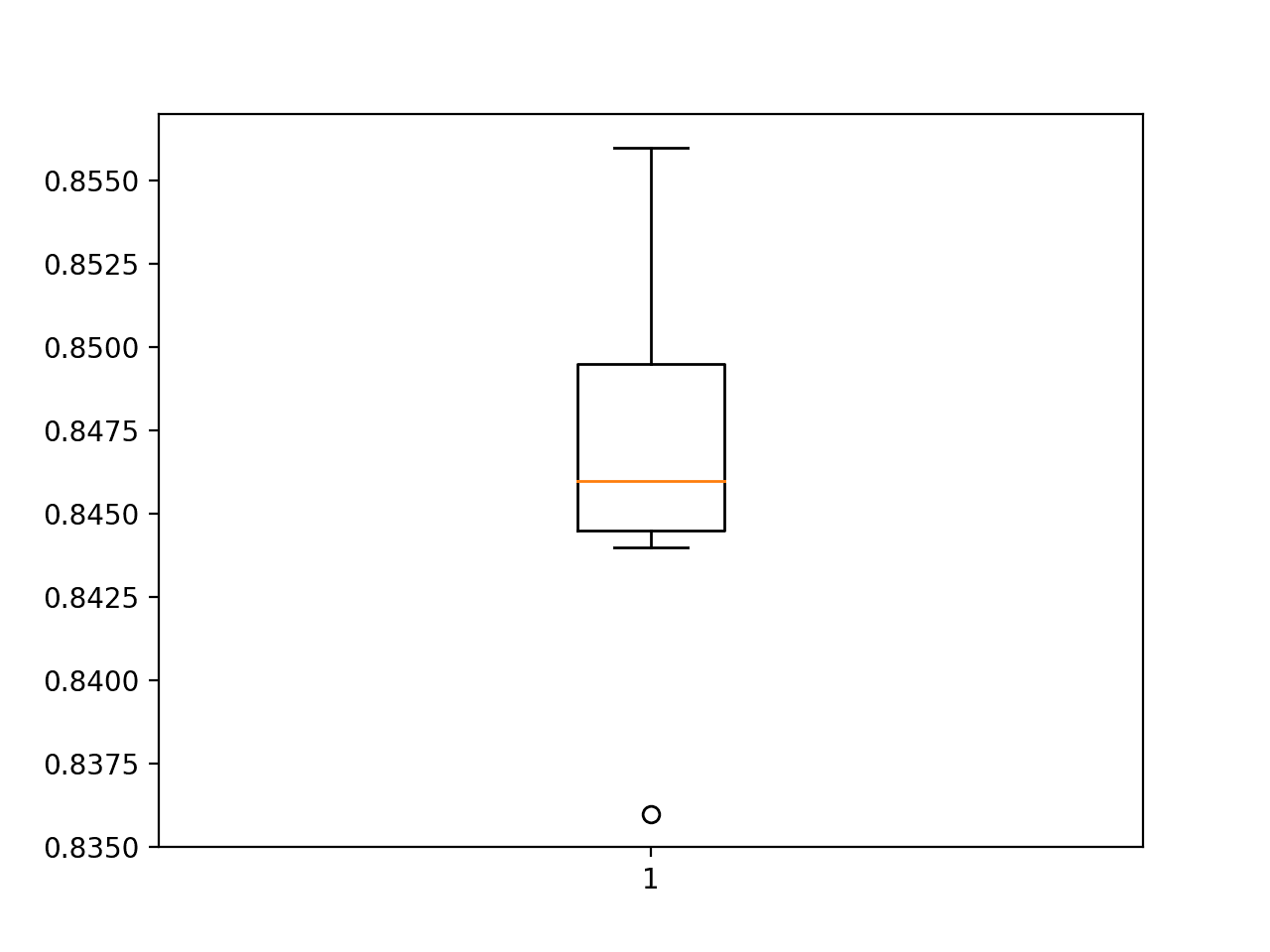
Score Over 10 Runs: 84.700 (0.531)
A box and whisker plot of the test accuracy scores is created showing the middle 50% of scores (called the interquartile range) denoted by the box ranges from a little below 84.5% to a little below 85%.
We can also see that the 83% value observed may be an outlier, given it is denoted as a dot.
Box and Whisker Plot of Test Accuracy of MLP on the Circles Problem
Study Test Accuracy vs Training Set Size
Given a fixed amount of statistical noise and a fixed but reasonably configured model, how many examples are required to learn the circles problem?
We can investigate this question by evaluating the performance of MLP models fit on training datasets of different size.
As a foundation, we can define a large number of examples that we believe would be far more than sufficient to learn the problem, such as 100,000. We can use this as an upper-bound on the number of training examples and use this many examples in the test set. We will define a model that performs well on this dataset as a model that has effectively learned the two circles problem.
We can then experiment by fitting models with different sized training datasets and evaluate their performance on the test set.
Too few examples will result in a low test accuracy, perhaps because the chosen model overfits the training set or the training set is not sufficiently representative of the problem.
Too many examples will result in good, but perhaps slightly lower than ideal test accuracy, perhaps because the chosen model does not have the capacity to learn the nuance of such a large training dataset, or the dataset is over-representative of the problem.
A line plot of training dataset size to model test accuracy should show an increasing trend to a point of diminishing returns and perhaps even a final slight drop in performance.
We can use the create_dataset() function defined in the previous section to create train and test datasets and set a default for the size of the test set argument to be 100,000 examples while allowing the size of the training set to be specified and vary with each call. Importantly, we want to use the same test set for each different sized training dataset.
We can create a new function to perform the repeated evaluation of a given model to account for the stochastic learning algorithm.
The evaluate_size() function below takes the size of the training set as an argument, as well as the number of repeats, that defaults to five to keep running time down. The create_dataset() function is created to create the train and test sets, and then the evaluate_model() function is called repeatedly to evaluate the model. The function then returns a list of scores for the repeats.
1
2
3
4
5
6
7
8
9
10
11
# repeated evaluation of mlp model with dataset of a given size
def evaluate_size(n_train,n_repeats=5):
# create dataset
trainX,trainy,testX,testy=create_dataset(n_train)
# repeat evaluation of model with dataset
scores=list()
for_inrange(n_repeats):
# evaluate model for size
score=evaluate_model(trainX,trainy,testX,testy)
scores.append(score)
returnscores
This function can then be called repeatedly. I would guess that somewhere between 1,000 and 10,000 examples of the problem would be sufficient to learn the problem, where sufficient means only small fractional differences in test accuracy.
Therefore, we will investigate training set sizes of 100, 1,000, 5,000, and 10,000 examples. The mean test accuracy will be reported for each test size to give an idea of progress.
1
2
3
4
5
6
7
8
9
10
11
# define dataset sizes to evaluate
sizes=[100,1000,5000,10000]
score_sets,means=list(),list()
forn_train insizes:
# repeated evaluate model with training set size
scores=evaluate_size(n_train)
score_sets.append(scores)
# summarize score for size
mean_score=mean(scores)
means.append(mean_score)
print('Train Size=%d, Test Accuracy %.3f'%(n_train,mean_score*100))
At the end of the run, a line plot will be created to show the relationship between train set size and model test set accuracy. We would expect to see an exponential curve from poor accuracy to a point of diminishing returns.
Box and whisker plots of the score distributions for each test set size are also created. We would expect to see a shrinking in the spread of test accuracy as the size of the training set is increased.
The complete example is listed below.
1
2
3
4
5
6
7
8
9
10
11
12
13
14
15
16
17
18
19
20
21
22
23
24
25
26
27
28
29
30
31
32
33
34
35
36
37
38
39
40
41
42
43
44
45
46
47
48
49
50
51
52
53
54
55
56
57
58
59
60
# study of training set size for an mlp on the circles problem
# repeated evaluation of mlp model with dataset of a given size
def evaluate_size(n_train,n_repeats=5):
# create dataset
trainX,trainy,testX,testy=create_dataset(n_train)
# repeat evaluation of model with dataset
scores=list()
for_inrange(n_repeats):
# evaluate model for size
score=evaluate_model(trainX,trainy,testX,testy)
scores.append(score)
returnscores
# define dataset sizes to evaluate
sizes=[100,1000,5000,10000]
score_sets,means=list(),list()
forn_train insizes:
# repeated evaluate model with training set size
scores=evaluate_size(n_train)
score_sets.append(scores)
# summarize score for size
mean_score=mean(scores)
means.append(mean_score)
print('Train Size=%d, Test Accuracy %.3f'%(n_train,mean_score*100))
# summarize relationship of train size to test accuracy
pyplot.plot(sizes,means,marker='o')
pyplot.show()
# plot distributions of test accuracy for train size
pyplot.boxplot(score_sets,labels=sizes)
pyplot.show()
Running the example may take a few minutes on modern hardware.
Note: Your results may vary given the stochastic nature of the algorithm or evaluation procedure, or differences in numerical precision. Consider running the example a few times and compare the average outcome.
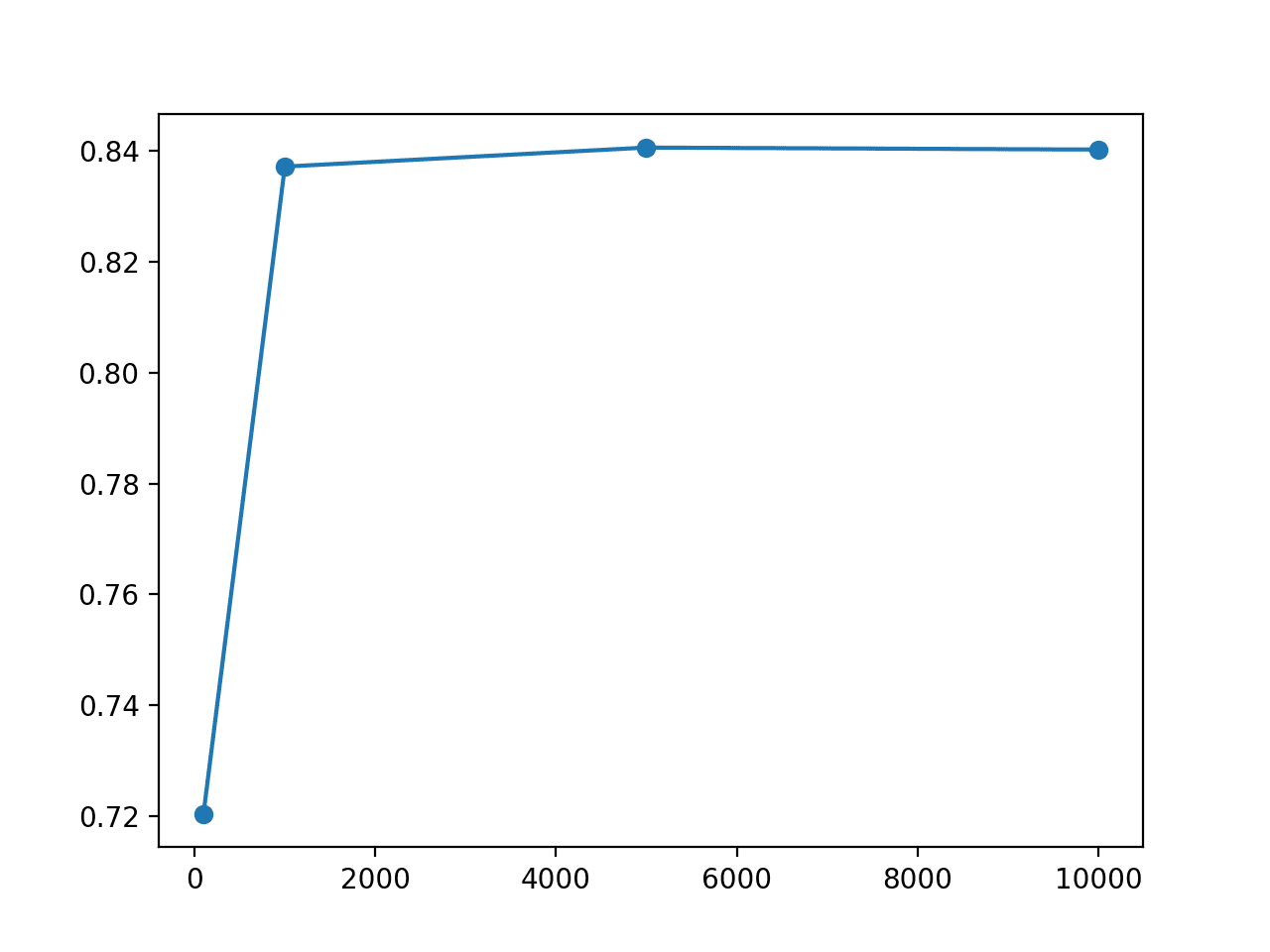
The mean model performance is reported for each training set size, showing a steady improvement in test accuracy as the training set is increased, as we expect. We also see a small drop in the average model performance from 5,000 to 10,000 examples, very likely highlighting that the variance in the data sample has exceeded the capacity of the chosen model configuration (number of layers and nodes).
1
2
3
4
Train Size=100, Test Accuracy 72.041
Train Size=1000, Test Accuracy 83.719
Train Size=5000, Test Accuracy 84.062
Train Size=10000, Test Accuracy 84.025
A line plot of test accuracy vs training set size is created.
We can see a sharp increase in test accuracy from 100 to 1,000 examples, after which performance appears to level off.
Line Plot of Training Set Size vs Test Set Accuracy for an MLP Model on the Circles Problem
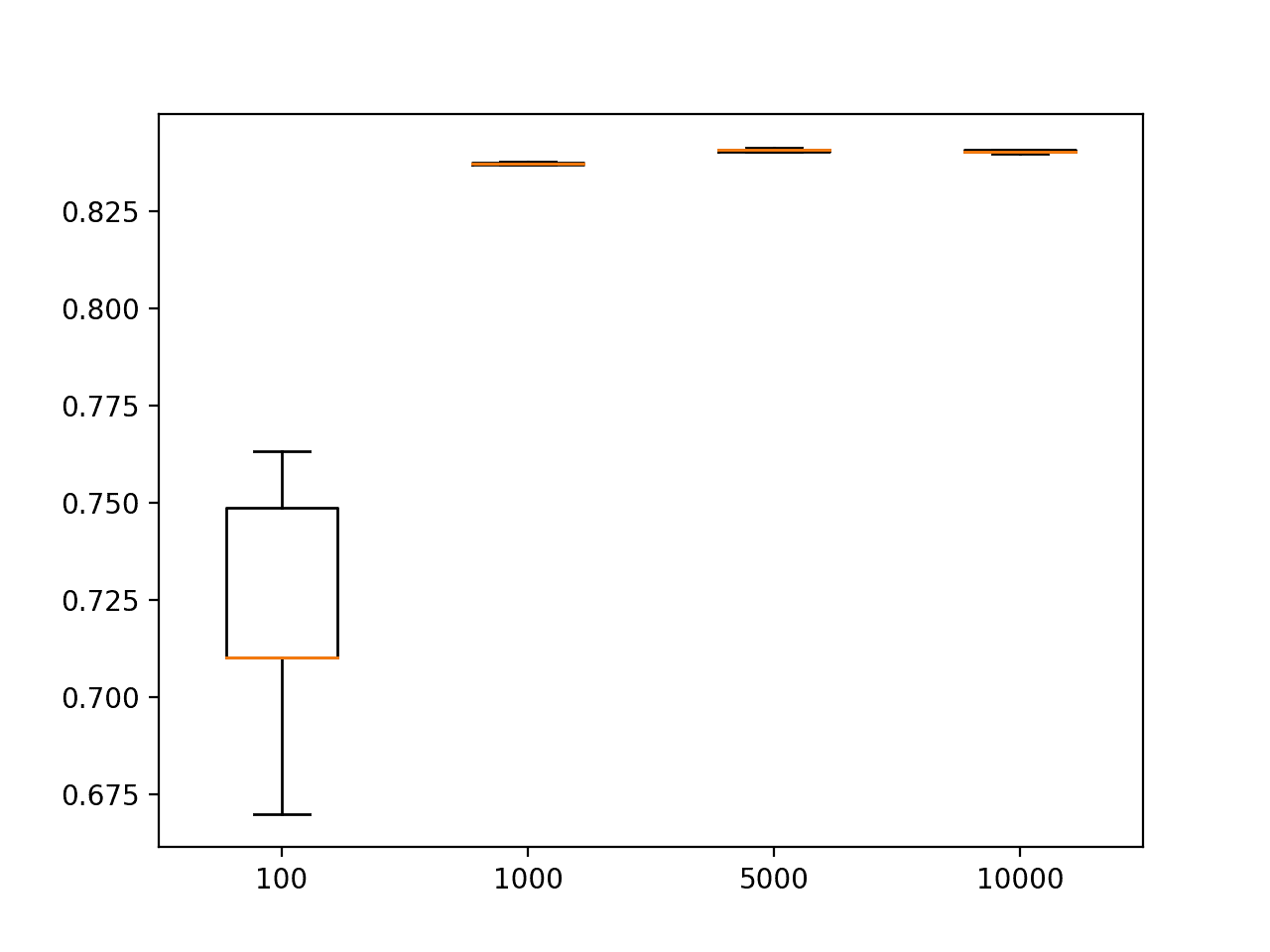
A box and whisker plot is created showing the distribution of test accuracy scores for each sized training dataset. As expected, we can see that the spread of test set accuracy scores shrinks dramatically as the training set size is increased, although remains small on the plot given the chosen scale.
Box and Whisker Plots of Test Set Accuracy of MLPs Trained With Different Sized Training Sets on the Circles Problem
The results suggest that the chosen MLP model configuration can learn the problem reasonably well with 1,000 examples, with quite modest improvements seen with 5,000 and 10,000 examples. Perhaps there is a sweet spot of 2,500 examples that results in an 84% test set accuracy with less than 5,000 examples.
The performance of neural networks can continually improve as more and more data is provided to the model, but the capacity of the model must be adjusted to support the increases in data. Eventually, there will be a point of diminishing returns where more data will not provide more insight into how to best model the mapping problem. For simpler problems, like two circles, this point will be reached sooner than in more complex problems, such as classifying photos of objects.
This study has highlighted a fundamental aspect of applied machine learning, specifically that you need enough examples of the problem to learn a useful approximation of the unknown underlying mapping function.
We almost never have an abundance of or too much training data. Therefore, our focus is often on how to most economically use available data and how to avoid overfitting the statistical noise present in the training dataset.
Study Test Set Size vs Test Set Accuracy
Given a fixed model and a fixed training dataset, how much test data is required to achieve an accurate estimate of the model performance?
We can investigate this question by fitting an MLP with a fixed sized training set and evaluating the model with different sized test sets.
We can use much the same strategy as the study in the previous section. We will fix the training set size at 1,000 examples as it resulted in a reasonably effective model with an estimated accuracy of about 83.7% when evaluated on 100,000 examples. We would expect that there is a smaller test set size that can reasonably approximate this value.
The create_dataset() function can be updated to specify the test set size and to use a default of 1,000 examples for the training set size. Importantly, the same 1,000 examples are used for the training set each time the size of the test set is varied.
We can use the same fit_model() function to fit the model. Because we’re using the same training dataset and varying the test dataset, we can create and fit the models once and re-use them for each differently sized test set. In this case, we will fit 10 models on the same training dataset to simulate 10 repeats.
Once fit, we can evaluate each of the models using a given sized test dataset. The evaluate_test_set_size() function below implements this behavior, returning a list of test set accuracy scores for the list of fit models and a given test set size.
1
2
3
4
5
6
7
8
9
10
# evaluate a test set of a given size on the fit models
def evaluate_test_set_size(models,n_test):
# create dataset
_,_,testX,testy=create_dataset(n_test)
scores=list()
formodel inmodels:
# evaluate the model
_,test_acc=model.evaluate(testX,testy,verbose=0)
scores.append(test_acc)
returnscores
We will evaluate four different sized test sets with 100, 1,000, 5,000, and 10,000 examples. We can then report the mean scores for each sized test set and create the same line and box and whisker plots.
1
2
3
4
5
6
7
8
9
10
11
12
13
14
15
16
17
# define test set sizes to evaluate
sizes=[100,1000,5000,10000]
score_sets,means=list(),list()
forn_test insizes:
# evaluate a test set of a given size on the models
scores=evaluate_test_set_size(models,n_test)
score_sets.append(scores)
# summarize score for size
mean_score=mean(scores)
means.append(mean_score)
print('Test Size=%d, Test Accuracy %.3f'%(n_test,mean_score*100))
# summarize relationship of test size to test accuracy
pyplot.plot(sizes,means,marker='o')
pyplot.show()
# plot distributions of test size to test accuracy
pyplot.boxplot(score_sets,labels=sizes)
pyplot.show()
Tying these elements together, the complete example is listed below.
1
2
3
4
5
6
7
8
9
10
11
12
13
14
15
16
17
18
19
20
21
22
23
24
25
26
27
28
29
30
31
32
33
34
35
36
37
38
39
40
41
42
43
44
45
46
47
48
49
50
51
52
53
54
55
56
57
58
59
60
61
62
63
# study of test set size for an mlp on the circles problem
# evaluate a test set of a given size on the models
scores=evaluate_test_set_size(models,n_test)
score_sets.append(scores)
# summarize score for size
mean_score=mean(scores)
means.append(mean_score)
print('Test Size=%d, Test Accuracy %.3f'%(n_test,mean_score*100))
# summarize relationship of test size to test accuracy
pyplot.plot(sizes,means,marker='o')
pyplot.show()
# plot distributions of test size to test accuracy
pyplot.boxplot(score_sets,labels=sizes)
pyplot.show()
Running the example reports the test set accuracy for each differently sized test set, averaged across the 10 models trained on the same dataset.
Note: Your results may vary given the stochastic nature of the algorithm or evaluation procedure, or differences in numerical precision. Consider running the example a few times and compare the average outcome.
If we take the result from the previous section of 83.7% when evaluated on 100,000 examples as an estimate of ground truth, then we can see that the smaller sized test sets vary above and below this estimate.
1
2
3
4
5
Fit 10 models
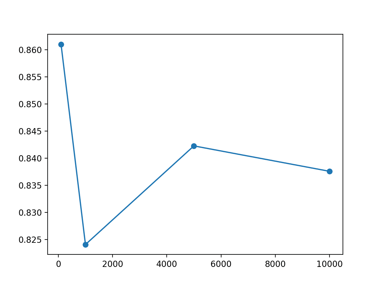
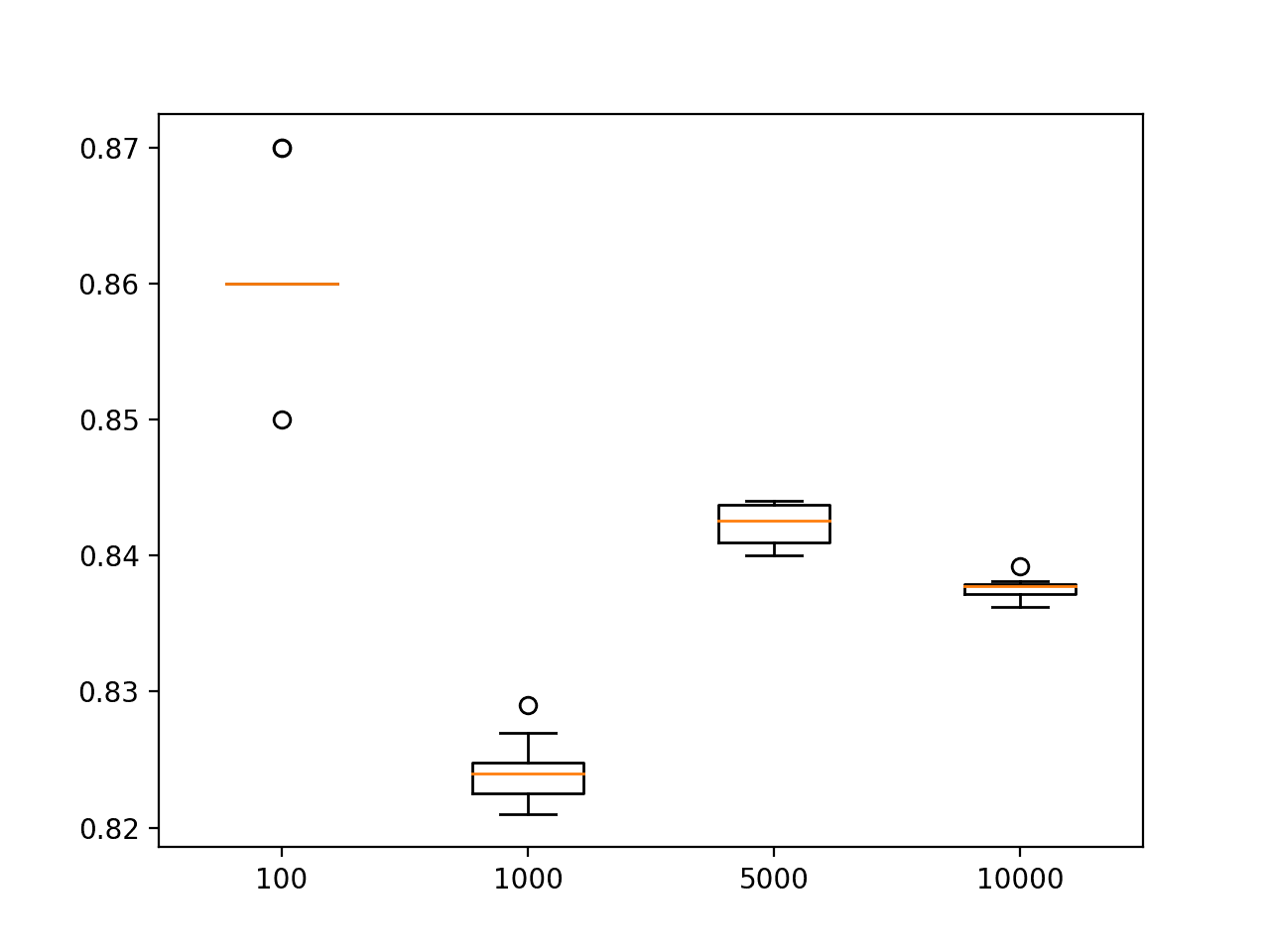
Test Size=100, Test Accuracy 86.100
Test Size=1000, Test Accuracy 82.410
Test Size=5000, Test Accuracy 84.228
Test Size=10000, Test Accuracy 83.760
A line plot of test set size vs test set accuracy is created.
The plot shows that smaller test set sizes of 100 and 1,000 examples overestimate and underestimate the accuracy of the model respectively. The results for a test set of 5,000 and 10,000 are a closer fit, the latter perhaps showing the best match.
This is surprising as a naive expectation might be that a test set of the same size as the training set would be a reasonable approximation of model accuracy, e.g. as though we performed a 50%/50% split of a 2,000 example dataset.
Line Plot of Test Set Size vs Test Set Accuracy for an MLP on the Circles Problem
A box and whisker plots show that the smaller test set demonstrates a large spread of scores, all of which are optimistic.
Box and Whisker Plot of the Distribution of Test set Accuracy for Different Test Set Sizes on the Circles Problem
It should be pointed out that we are not reporting on the average performance of the chosen model on random examples drawn from the domain. The model and the examples are fixed and the only source of variation is from the learning algorithm.
The study demonstrates how sensitive the estimated accuracy of the model is to the size of the test dataset. This is an important consideration as often little thought is given to the test set size, using a familiar split of 70%/30% or 80%/20% for train/test splits.
As pointed out in the previous section, we often rarely have enough data, and spending a precious portion of the data on a test or even validation dataset is often rarely considered in any great depth. The results highlight how important cross-validation methods such as leave-one-out cross-validation are, allowing the model to make a test prediction for each example in the dataset, yet come at such a great computational cost, requiring almost one model to be trained for each example in the dataset.
In practice, we must struggle with a training dataset that is too small to learn the unknown underlying mapping function and a test dataset that is too small to reasonably approximate the performance of the model on the problem.
Further Reading
This section provides more resources on the topic if you are looking to go deeper.
In this tutorial, you discovered that in practice, we don’t have enough data to learn the mapping function or to evaluate models, yet supervised learning algorithms like neural networks remain remarkably effective.
Specifically, you learned:
How to analyze the two circles classification problem and measure the variance introduced by the neural network learning algorithm.
How changes in the size of a training dataset directly impact the quality of the mapping function approximated by neural networks.
How the changes in the size of a test dataset directly impact the quality of the estimated in the performance of a fit neural network model.
Do you have any questions?
Ask your questions in the comments below and I will do my best to answer.
I have dataset that contains records of transactions for 2 years, I decided to use the last two months from that distribution as test set, and the remaining for train and dev sets. Is that a good idea? I am also aware of the possible absence of labels in the test set. The problem is for multi-label classification.
Is there any specific reason why there is no possibility to set a pseudo random generator seedat the initialization of ANN? (Just as we do for data splitting, or for many ML algorithms). I suppose that initial ANN weights could use this seed and SGD as well. Do you know the reason why the implementations neglect/omit this feature?
Thanks so much for this detailed tutorial.
May I please request any information that you may have on dimensions vs accuracy and at what point the gains in accuracy diminish with regards to dimensions?
Hello, is there any correlation between the number of features with the DL model’s training or testing time? Will training a model with 50 features take longer than training a model with 10 features? Thanks
Hello,
I wanted to ask for binary classification for 2000 samples of my dataset…each sample has 475 data points…my algorithm trains very fast on jupyter notebook and shows 90% accuracy… what am i doing wrong? it trains within one minute for 50 epochs.. i am using keras and tensorflow…. i thought neural networks take lot of time to train…i am new to this topic so pardon me if it seems stupid… am i9 doing something wrong?
I’m currently working on an image classification problem (binary). I have an equal amount of images for both classes, but in reality, the possibility of the occurrence of one of the classes is much lower than the other. Is there a way to reflect this in the training process? Additionally, I also have the same question as most others here: How to find out how much data is enough to prevent overfitting? At present, I have ~250 original images for each class and I have already implemented augmentation to triple the size to ~750 in each class. How to find out how many more images are required? Thanks in advance.
Yes, ideally the training dataset and test dataset would be representative of the underlying problem. Perhaps you can gain a different sample that better matches a random sample from the domain?
I am currently working on crop recommendation problem where i am considering 7 features to predict most suitable crop. I am having dataset of 2200 rows. predciting for 22 types of crop. how to know if this is sufficient for prediction.or if i need more data instance if yes than please help me how to increase the size of dataset in case of numerical dataset
Fatma Nihal Urasoğlu AkçayOctober 19, 2021 at 12:02 am#
Thank you for the tutorial. I have 5 different classes to determine using CNN and in my datasets there are different amount of images. Does this effect badly for learning of CNN or all the datasets must have exact the same amount of images?
As long as the number in each class are roughly the same, it should not matter. If you have one class that has 100 times more image than another, the model may blindly select the majority class and still get a good accuracy score. That’s the problem of imbalanced data set. If your case is not that exaggerated, it should be OK.
I’m currently working on a text classification problem where I have lots of raw data but none of them are labeled. Thus, I’m labeling the data as I fine-tune a transformer model. I’m versioning the dataset but the dataset with 150 samples (version 3) outperforms the latest dataset that has 350 samples.
The difference in performance is around 5%, I’ve been monitoring a few metrics (accuracy, f1, recall and precision, and Matthews correlation) and the performance drops drastically after I continue to add more labeled data to the dataset-3.
The splits were stratified and the test set ratio was 20%. My conclusion was overestimation because of the test set size, would there be another case to consider?


Thanks Jason as always for your great article.
I have a question on small data set on binary classification, what is the best pre-processing implementation we would use?
Do we need to zero centering our data or just normalisation of our data set?
pardon my question if not clear enough.
Thanks
Try a range of preprocessing steps and see which results in faster learning or better performance.
I have dataset that contains records of transactions for 2 years, I decided to use the last two months from that distribution as test set, and the remaining for train and dev sets. Is that a good idea? I am also aware of the possible absence of labels in the test set. The problem is for multi-label classification.
Thanks!
I recommend testing different amount of history input to discover what works best for your specific dataset.
Good morning Jason,
Thank you for this post!
Is there any specific reason why there is no possibility to set a pseudo random generator seedat the initialization of ANN? (Just as we do for data splitting, or for many ML algorithms). I suppose that initial ANN weights could use this seed and SGD as well. Do you know the reason why the implementations neglect/omit this feature?
Best regards!
Yes, it is a bad strategy:
https://machinelearningmastery.com/randomness-in-machine-learning/
Instead, we control for the stochastic nature of the learning algorithm using repeated model evaluations.
https://machinelearningmastery.com/evaluate-skill-deep-learning-models/
Hi
Thanks so much for this detailed tutorial.
May I please request any information that you may have on dimensions vs accuracy and at what point the gains in accuracy diminish with regards to dimensions?
Thanks
Vel
It depends on the model and dataset.
You can run a study with your own model and dataset to discover the relationship.
Hello, is there any correlation between the number of features with the DL model’s training or testing time? Will training a model with 50 features take longer than training a model with 10 features? Thanks
Yes, more features means a slower model.
Hello,
I wanted to ask for binary classification for 2000 samples of my dataset…each sample has 475 data points…my algorithm trains very fast on jupyter notebook and shows 90% accuracy… what am i doing wrong? it trains within one minute for 50 epochs.. i am using keras and tensorflow…. i thought neural networks take lot of time to train…i am new to this topic so pardon me if it seems stupid… am i9 doing something wrong?
What is the problem exactly?
It trains fast?
It achieves a score of 90% accuracy?
I’m currently working on an image classification problem (binary). I have an equal amount of images for both classes, but in reality, the possibility of the occurrence of one of the classes is much lower than the other. Is there a way to reflect this in the training process? Additionally, I also have the same question as most others here: How to find out how much data is enough to prevent overfitting? At present, I have ~250 original images for each class and I have already implemented augmentation to triple the size to ~750 in each class. How to find out how many more images are required? Thanks in advance.
Yes, ideally the training dataset and test dataset would be representative of the underlying problem. Perhaps you can gain a different sample that better matches a random sample from the domain?
I am currently working on crop recommendation problem where i am considering 7 features to predict most suitable crop. I am having dataset of 2200 rows. predciting for 22 types of crop. how to know if this is sufficient for prediction.or if i need more data instance if yes than please help me how to increase the size of dataset in case of numerical dataset
Perhaps evaluate a few models and discover how useful the available data can be in developing a predictive model.
Thank you very much for the nice example. I learned how size of the training data is important.
You’re welcome.
Thank you for the tutorial. I have 5 different classes to determine using CNN and in my datasets there are different amount of images. Does this effect badly for learning of CNN or all the datasets must have exact the same amount of images?
As long as the number in each class are roughly the same, it should not matter. If you have one class that has 100 times more image than another, the model may blindly select the majority class and still get a good accuracy score. That’s the problem of imbalanced data set. If your case is not that exaggerated, it should be OK.
Thanks for the detailed example.
I’m currently working on a text classification problem where I have lots of raw data but none of them are labeled. Thus, I’m labeling the data as I fine-tune a transformer model. I’m versioning the dataset but the dataset with 150 samples (version 3) outperforms the latest dataset that has 350 samples.
The difference in performance is around 5%, I’ve been monitoring a few metrics (accuracy, f1, recall and precision, and Matthews correlation) and the performance drops drastically after I continue to add more labeled data to the dataset-3.
The splits were stratified and the test set ratio was 20%. My conclusion was overestimation because of the test set size, would there be another case to consider?
Hi Efe…Thank you for your feedback! The following is a great place to start in order to improve performance of your models:
https://machinelearningmastery.com/better-deep-learning-neural-networks-crash-course/