Leveraging ANOVA and Kruskal-Wallis Tests to Analyze the Impact of the Great Recession on Housing Prices

By Vinod Chugani on March 28, 2024 in Data Science 0

In the world of real estate, numerous factors influence property prices. The economy, market demand, location, and even the year a property is sold can play significant roles. The years 2007 to 2009 marked a tumultuous time for the US housing market. This period, often referred to as the Great Recession, saw a drastic decline in home values, a surge in foreclosures, and widespread financial market turmoil. The impact of the recession on housing prices was profound, with many homeowners finding themselves in homes that were worth less than their mortgages. The ripple effect of this downturn was felt across the country, with some areas experiencing sharper declines and slower recoveries than others.

Given this backdrop, it’s particularly intriguing to analyze housing data from Ames, Iowa, as the dataset spans from 2006 to 2010, encapsulating the height and aftermath of the Great Recession. Does the year of sale, amidst such economic volatility, influence the sales price in Ames? In this post, you’ll delve deep into the Ames Housing dataset to explore this query using Exploratory Data Analysis (EDA) and two statistical tests: ANOVA and the Kruskal-Wallis Test.

Let’s get started.

Leveraging ANOVA and Kruskal-Wallis Tests to Analyze the Impact of the Great Recession on Housing Prices
Photo by Sharissa Johnson. Some rights reserved.

Overview

This post is divided into three parts; they are:

EDA: Visual Insights
Assessing Variability in Sales Prices Across Years Using ANOVA
Kruskal-Wallis Test: A Non-Parametric Alternative to ANOVA

EDA: Visual Insights

To begin, let’s load the Ames Housing dataset and compare different years of sale against the dependent variable: the sales price.

# Importing the essential libraries
import pandas as pd
import seaborn as sns
import matplotlib.pyplot as plt

# Load the dataset
Ames = pd.read_csv('Ames.csv')

# Convert 'YrSold' to a categorical variable
Ames['YrSold'] = Ames['YrSold'].astype('category')

plt.figure(figsize=(10, 6))
sns.boxplot(x=Ames['YrSold'], y=Ames['SalePrice'], hue=Ames['YrSold'])
plt.title('Boxplot of Sales Prices by Year', fontsize=18)
plt.xlabel('Year Sold', fontsize=15)
plt.ylabel('Sales Price (US$)', fontsize=15)
plt.legend('')
plt.show()

# Importing the essential libraries

import pandas as pd

import seaborn as sns

import matplotlib.pyplot as plt

# Load the dataset

Ames = pd.read_csv('Ames.csv')

# Convert 'YrSold' to a categorical variable

Ames['YrSold'] = Ames['YrSold'].astype('category')

plt.figure(figsize=(10, 6))

sns.boxplot(x=Ames['YrSold'], y=Ames['SalePrice'], hue=Ames['YrSold'])

plt.title('Boxplot of Sales Prices by Year', fontsize=18)

plt.xlabel('Year Sold', fontsize=15)

plt.ylabel('Sales Price (US$)', fontsize=15)

plt.legend('')

plt.show()

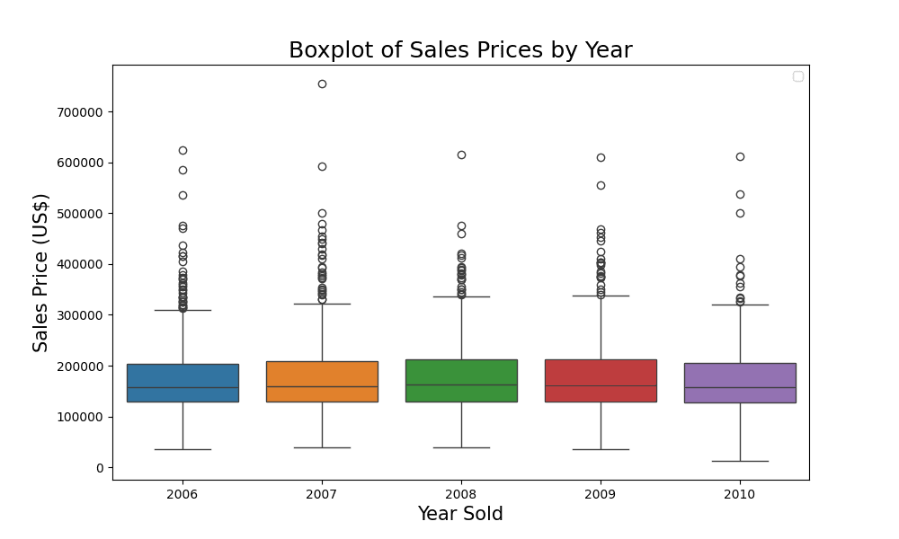
Comparing the trend of sales prices

From the boxplot, you can observe that the sales prices were quite consistent across different years because each year looks alike. Let’s take a closer look using the groupby function in pandas.

# Calculating mean and median sales price by year
summary_table = Ames.groupby('YrSold')['SalePrice'].agg(['mean', 'median'])

# Rounding the values for better presentation
summary_table = summary_table.round(2)
print(summary_table)

# Calculating mean and median sales price by year

summary_table = Ames.groupby('YrSold')['SalePrice'].agg(['mean', 'median'])

# Rounding the values for better presentation

summary_table = summary_table.round(2)

print(summary_table)

The output is:

             mean    median
YrSold                     
2006    176615.62  157000.0
2007    179045.08  159000.0
2008    178170.02  162700.0
2009    180387.64  162000.0
2010    173971.67  157900.0

mean median

YrSold

2006 176615.62 157000.0

2007 179045.08 159000.0

2008 178170.02 162700.0

2009 180387.64 162000.0

2010 173971.67 157900.0

From the table, you can make the following observations:

The mean sales price was the highest in 2009 at approximately \$180,388, while it was the lowest in 2010 at around \$173,972.
The median sales price was the highest in 2008 at \$162,700 and the lowest in 2006 at \$157,000.
Even though the mean and median sales prices are close in value for each year, there are slight variations. This suggests that while there might be some outliers influencing the mean, they are not extremely skewed.
Over the five years, there doesn’t seem to be a consistent upward or downward trend in sales prices, which is interesting given the larger economic context (the Great Recession) during this period.

This table, combined with the boxplot, gives a comprehensive view of the distribution and central tendency of sales prices across the years. It sets the stage for deeper statistical analysis to determine if the observed differences (or lack thereof) are statistically significant.

Kick-start your project with my book The Beginner’s Guide to Data Science. It provides self-study tutorials with working code.

Assessing Variability in Sales Prices Across Years Using ANOVA

ANOVA (Analysis of Variance) helps us test if there are any statistically significant differences between the means of three or more independent groups. Its null hypothesis is that the means of all groups are equal. This can be considered as a version of t-test to support more than two groups. It makes use of the F-test statistic to check if the variance ($\sigma^2$) is different within each group compared to across all groups.

The hypothesis setup is:

$H_0$: The means of sales price for all years are equal.
$H_1$: At least one year has a different mean sales price.

You can run your test using the scipy.stats library as follows:

# Import an additional library
import scipy.stats as stats

# Perform the ANOVA
f_value, p_value = stats.f_oneway(*[Ames['SalePrice'][Ames['YrSold'] == year]
                                    for year in Ames['YrSold'].unique()])

print(f_value, p_value)

# Import an additional library

import scipy.stats as stats

# Perform the ANOVA

f_value, p_value = stats.f_oneway(*[Ames['SalePrice'][Ames['YrSold'] == year]

for year in Ames['YrSold'].unique()])

print(f_value, p_value)

The two values are:

0.4478735462379817 0.774024927554816

1	0.4478735462379817 0.774024927554816

The results of the ANOVA test are:

F-value: 0.4479
p-value: 0.7740

Given the high p-value (greater than a common significance level of 0.05), you cannot reject the null hypothesis ($H_0$). This suggests that there are no statistically significant differences between the means of sales price for the different years present in the dataset.

While your ANOVA results provide insights into the equality of means across different years, it’s essential to ensure that the assumptions underlying the test have been met. Let’s delve into verifying the 3 assumptions of ANOVA tests to validate your findings.

Assumption 1: Independence of Observations. Since each observation (house sale) is independent of another, this assumption is met.

Assumption 2: Normality of the Residuals. For ANOVA to be valid, the residuals from the model should approximately follow a normal distribution since this is the model behind F-test. You can check this both visually and statistically.

Visual assessment can be done using a QQ plot:

# Import an additional library
import statsmodels.api as sm

# Fit an ordinary least squares model and get residuals
model = sm.OLS(Ames['SalePrice'], Ames['YrSold'].astype('int')).fit()
residuals = model.resid

# Plot QQ plot
sm.qqplot(residuals, line='s')
plt.title('Normality Assessment of Residuals via QQ Plot', fontsize=18)
plt.xlabel('Theoretical Quantiles', fontsize=15)
plt.ylabel('Sample Residual Quantiles', fontsize=15)
plt.grid(True, which='both', linestyle='--', linewidth=0.5)
plt.show()

# Import an additional library

import statsmodels.api as sm

# Fit an ordinary least squares model and get residuals

model = sm.OLS(Ames['SalePrice'], Ames['YrSold'].astype('int')).fit()

residuals = model.resid

# Plot QQ plot

sm.qqplot(residuals, line='s')

plt.title('Normality Assessment of Residuals via QQ Plot', fontsize=18)

plt.xlabel('Theoretical Quantiles', fontsize=15)

plt.ylabel('Sample Residual Quantiles', fontsize=15)

plt.grid(True, which='both', linestyle='--', linewidth=0.5)

plt.show()

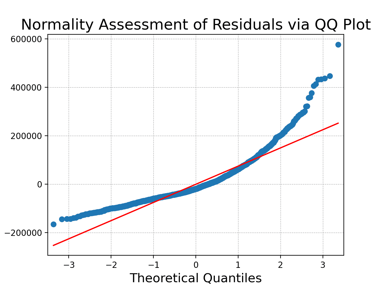
The QQ Plot presented above serves as a valuable visual tool to assess the normality of your dataset’s residuals, offering insights into how well the observed data aligns with the theoretical expectations of a normal distribution. In this plot, each point represents a pair of quantiles: one from the residuals of your data and the other from the standard normal distribution. Ideally, if your data perfectly followed a normal distribution, all the points on the QQ Plot would fall precisely along the red 45-degree reference line. The plot illustrates deviations from the 45-degree reference line, suggesting potential deviations from normality.

Statistical assessment can be done using the Shapiro-Wilk Test, which provides a formal method to test for normality. The null hypothesis of the test is that the data follows a normal distribution. This test also available in SciPy:

#Import shapiro from scipy.stats package
from scipy.stats import shapiro

# Shapiro-Wilk Test
shapiro_stat, shapiro_p = shapiro(residuals)
print(f"Shapiro-Wilk Test Statistic: {shapiro_stat}\nP-value: {shapiro_p}")

#Import shapiro from scipy.stats package

from scipy.stats import shapiro

# Shapiro-Wilk Test

shapiro_stat, shapiro_p = shapiro(residuals)

print(f"Shapiro-Wilk Test Statistic: {shapiro_stat}\nP-value: {shapiro_p}")

The output is:

Shapiro-Wilk Test Statistic: 0.8774482011795044
P-value: 4.273399796804962e-41

1 2	Shapiro-Wilk Test Statistic: 0.8774482011795044 P-value: 4.273399796804962e-41

A low p-value (typically ) suggests rejecting the null hypothesis, indicating that the residuals do not follow a normal distribution. This indicates a violation of the second assumption of ANOVA, which requires that the residuals be normally distributed. Both the QQ plot and the Shapiro-Wilk test converge on the same conclusion: the residuals do not strictly adhere to a normal distribution. Hence, the result of the ANOVA may not be valid.

Assumption 3: Homogeneity of Variances. The variances of the groups (years) should be approximately equal. This happens to be the null hypothesis of Levene’s test. Hence you can use it to verify:

# Check for equal variances using Levene's test
levene_stat, levene_p = stats.levene(*[Ames['SalePrice'][Ames['YrSold'] == year]
                                      for year in Ames['YrSold'].unique()])

print(f"Levene's Test Statistic: {levene_stat}\nP-value: {levene_p}")

# Check for equal variances using Levene's test

levene_stat, levene_p = stats.levene(*[Ames['SalePrice'][Ames['YrSold'] == year]

for year in Ames['YrSold'].unique()])

print(f"Levene's Test Statistic: {levene_stat}\nP-value: {levene_p}")

The output is:

Levene's Test Statistic: 0.2514412478357097
P-value: 0.9088910499612235

1 2	Levene's Test Statistic: 0.2514412478357097 P-value: 0.9088910499612235

Given the high p-value of from Levene’s test, you cannot reject the null hypothesis, indicating that the variances of sales prices across different years are statistically homogeneous, satisfying the third key assumption for ANOVA.

Putting all together, the following code runs the ANOVA test and verifies the three assumptions:

# Importing the essential libraries
import pandas as pd
import scipy.stats as stats
import matplotlib.pyplot as plt
import statsmodels.api as sm
from scipy.stats import shapiro

# Load the dataset
Ames = pd.read_csv('Ames.csv')

# Perform the ANOVA
f_value, p_value = stats.f_oneway(*[Ames['SalePrice'][Ames['YrSold'] == year]
                                    for year in Ames['YrSold'].unique()])
print("F-value:", f_value)
print("p-value:", p_value)

# Fit an ordinary least squares model and get residuals
model = sm.OLS(Ames['SalePrice'], Ames['YrSold'].astype('int')).fit()
residuals = model.resid

# Plot QQ plot
sm.qqplot(residuals, line='s')
plt.title('Normality Assessment of Residuals via QQ Plot', fontsize=18)
plt.xlabel('Theoretical Quantiles', fontsize=15)
plt.ylabel('Sample Residual Quantiles', fontsize=15)
plt.grid(True, which='both', linestyle='--', linewidth=0.5)
plt.show()

# Shapiro-Wilk Test
shapiro_stat, shapiro_p = shapiro(residuals)
print(f"Shapiro-Wilk Test Statistic: {shapiro_stat}\nP-value: {shapiro_p}")

# Check for equal variances using Levene's test
levene_stat, levene_p = stats.levene(*[Ames['SalePrice'][Ames['YrSold'] == year]
                                      for year in Ames['YrSold'].unique()])

print(f"Levene's Test Statistic: {levene_stat}\nP-value: {levene_p}")

# Importing the essential libraries

import pandas as pd

import scipy.stats as stats

import matplotlib.pyplot as plt

import statsmodels.api as sm

from scipy.stats import shapiro

# Load the dataset

Ames = pd.read_csv('Ames.csv')

# Perform the ANOVA

f_value, p_value = stats.f_oneway(*[Ames['SalePrice'][Ames['YrSold'] == year]

for year in Ames['YrSold'].unique()])

print("F-value:", f_value)

print("p-value:", p_value)

# Fit an ordinary least squares model and get residuals

model = sm.OLS(Ames['SalePrice'], Ames['YrSold'].astype('int')).fit()

residuals = model.resid

# Plot QQ plot

sm.qqplot(residuals, line='s')

plt.title('Normality Assessment of Residuals via QQ Plot', fontsize=18)

plt.xlabel('Theoretical Quantiles', fontsize=15)

plt.ylabel('Sample Residual Quantiles', fontsize=15)

plt.grid(True, which='both', linestyle='--', linewidth=0.5)

plt.show()

# Shapiro-Wilk Test

shapiro_stat, shapiro_p = shapiro(residuals)

print(f"Shapiro-Wilk Test Statistic: {shapiro_stat}\nP-value: {shapiro_p}")

# Check for equal variances using Levene's test

levene_stat, levene_p = stats.levene(*[Ames['SalePrice'][Ames['YrSold'] == year]

for year in Ames['YrSold'].unique()])

print(f"Levene's Test Statistic: {levene_stat}\nP-value: {levene_p}")

Kruskal-Wallis Test: A Non-Parametric Alternative to ANOVA

The Kruskal-Wallis test is a non-parametric method used to compare the median values of three or more independent groups, making it a suitable alternative to the one-way ANOVA (especially when assumptions of ANOVA are not met).

Non-parametric statistics are a class of statistical methods that do not make explicit assumptions about the underlying distribution of the data. In contrast to parametric tests, which assume a specific distribution (e.g., normal distribution in assumption 2 above), non-parametric tests are more flexible and can be applied to data that may not meet the stringent assumptions of parametric methods. Non-parametric tests are particularly useful when dealing with ordinal or nominal data, as well as data that might exhibit skewness or heavy tails. These tests focus on the order or rank of values rather than the specific values themselves. Non-parametric tests, including the Kruskal-Wallis test, offer a flexible and distribution-free approach to statistical analysis, making them suitable for a wide range of data types and situations.

The hypothesis setup under Kruskal-Wallis test is:

$H_0$: The distributions of the sales price for all years are identical.
$H_1$: At least one year has a different distribution of sales price.

You can run Kruskal-Wallis test using SciPy, as follows:

# Perform the Kruskal-Wallis H-test
H_statistic, kruskal_p_value = stats.kruskal(*[Ames['SalePrice'][Ames['YrSold'] == year]
                                               for year in Ames['YrSold'].unique()])

print(H_statistic, kruskal_p_value)

# Perform the Kruskal-Wallis H-test

H_statistic, kruskal_p_value = stats.kruskal(*[Ames['SalePrice'][Ames['YrSold'] == year]

for year in Ames['YrSold'].unique()])

print(H_statistic, kruskal_p_value)

The output is:

2.1330989438609236 0.7112941815590765

1	2.1330989438609236 0.7112941815590765

The results of the Kruskal-Wallis test are:

H-Statistic: 2.133
p-value: 0.7113

Note: The Kruskal-Wallis test doesn’t specifically test for differences in means (like ANOVA does), but rather for differences in distributions. This can include differences in medians, shapes, and spreads.

Given the high p-value (greater than a common significance level of 0.05), you cannot reject the null hypothesis. This suggests that there are no statistically significant differences in the median sales prices for the different years present in the dataset when using the Kruskal-Wallis test. Let’s delve into verifying the 3 assumptions of the Kruskal-Wallis test to validate your findings.

Assumption 1: Independence of Observations. This remains the same as for ANOVA; each observation is independent of another.

Assumption 2: The Response Variable Should be Ordinal, Interval, or Ratio. The sales price is a ratio variable, so this assumption is met.

Assumption 3: The Distributions of the Response Variable Should be the Same for All Groups. This can be validated using both visual and numerical methods.

# Plot histograms of Sales Price for each year
fig, axes = plt.subplots(nrows=5, ncols=1, figsize=(12, 8), sharex=True)

for idx, year in enumerate(sorted(Ames['YrSold'].unique())):
    sns.histplot(Ames[Ames['YrSold'] == year]['SalePrice'], kde=True, ax=axes[idx], color='skyblue')
    axes[idx].set_title(f'Distribution of Sales Prices for Year {year}', fontsize=16)
    axes[idx].set_ylabel('Frequency', fontsize=14)
    if idx == 4:
        axes[idx].set_xlabel('Sales Price', fontsize=15)
    else:
        axes[idx].set_xlabel('')

plt.tight_layout()
plt.show()

# Plot histograms of Sales Price for each year

fig, axes = plt.subplots(nrows=5, ncols=1, figsize=(12, 8), sharex=True)

for idx, year in enumerate(sorted(Ames['YrSold'].unique())):

sns.histplot(Ames[Ames['YrSold'] == year]['SalePrice'], kde=True, ax=axes[idx], color='skyblue')

axes[idx].set_title(f'Distribution of Sales Prices for Year {year}', fontsize=16)

axes[idx].set_ylabel('Frequency', fontsize=14)

if idx == 4:

axes[idx].set_xlabel('Sales Price', fontsize=15)

else:

axes[idx].set_xlabel('')

plt.tight_layout()

plt.show()

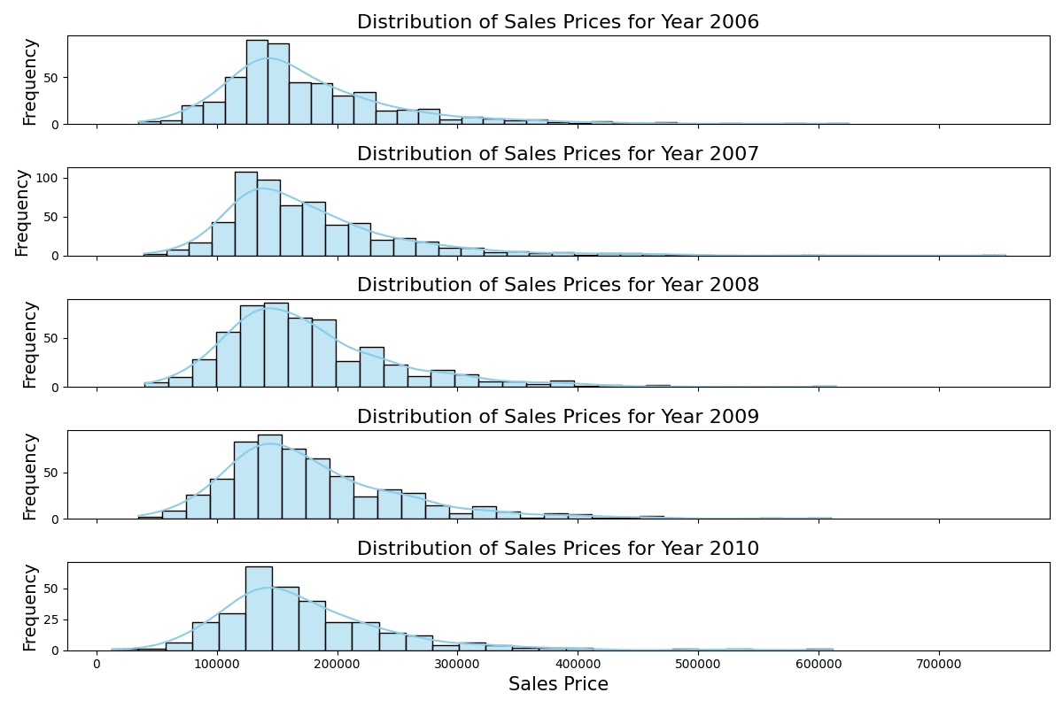
Distribution of sales prices of different years

The stacked histograms indicate consistent distributions of sales prices across the years, with each year displaying a similar range and peak despite slight variations in frequency.

Furthermore, you can conduct pairwise Kolmogorov-Smirnov tests, which is a non-parametric test to compare the similarity of two probability distributions. It is available in SciPy. You can use the version that the null hypothesis is the two distributions equal, and the alternative hypothesis is not equal:

# Run KS Test from scipy.stats
from scipy.stats import ks_2samp
results = {}
for i, year1 in enumerate(sorted(Ames['YrSold'].unique())):
    for j, year2 in enumerate(sorted(Ames['YrSold'].unique())):
        if i < j:
            ks_stat, ks_p = ks_2samp(Ames[Ames['YrSold'] == year1]['SalePrice'], 
                                     Ames[Ames['YrSold'] == year2]['SalePrice'])
            results[f"{year1} vs {year2}"] = (ks_stat, ks_p)

# Convert the results into a DataFrame for tabular representation
ks_df = pd.DataFrame(results).transpose()
ks_df.columns = ['KS Statistic', 'P-value']
ks_df.reset_index(inplace=True)
ks_df.rename(columns={'index': 'Years Compared'}, inplace=True)

print(ks_df)

# Run KS Test from scipy.stats

from scipy.stats import ks_2samp

results = {}

for i, year1 in enumerate(sorted(Ames['YrSold'].unique())):

for j, year2 in enumerate(sorted(Ames['YrSold'].unique())):

if i < j:

ks_stat, ks_p = ks_2samp(Ames[Ames['YrSold'] == year1]['SalePrice'],

Ames[Ames['YrSold'] == year2]['SalePrice'])

results[f"{year1} vs {year2}"] = (ks_stat, ks_p)

# Convert the results into a DataFrame for tabular representation

ks_df = pd.DataFrame(results).transpose()

ks_df.columns = ['KS Statistic', 'P-value']

ks_df.reset_index(inplace=True)

ks_df.rename(columns={'index': 'Years Compared'}, inplace=True)

print(ks_df)

This shows:

  Years Compared  KS Statistic   P-value
0   2006 vs 2007      0.038042  0.798028
1   2006 vs 2008      0.052802  0.421325
2   2006 vs 2009      0.062235  0.226623
3   2006 vs 2010      0.040006  0.896946
4   2007 vs 2008      0.039539  0.732841
5   2007 vs 2009      0.044231  0.586558
6   2007 vs 2010      0.051508  0.620135
7   2008 vs 2009      0.032488  0.908322
8   2008 vs 2010      0.052752  0.603031
9   2009 vs 2010      0.053236  0.586128

Years Compared KS Statistic P-value

0 2006 vs 2007 0.038042 0.798028

1 2006 vs 2008 0.052802 0.421325

2 2006 vs 2009 0.062235 0.226623

3 2006 vs 2010 0.040006 0.896946

4 2007 vs 2008 0.039539 0.732841

5 2007 vs 2009 0.044231 0.586558

6 2007 vs 2010 0.051508 0.620135

7 2008 vs 2009 0.032488 0.908322

8 2008 vs 2010 0.052752 0.603031

9 2009 vs 2010 0.053236 0.586128

While we satisfied only 2 out of the 3 assumptions for ANOVA, we have met all the necessary criteria for the Kruskal-Wallis test. The pairwise Kolmogorov-Smirnov tests indicate that the distributions of sales prices across different years are remarkably consistent. Specifically, the high p-values (all greater than the common significance level of 0.05) imply that there isn’t enough evidence to reject the hypothesis that the sales prices for each year come from the same distribution. These findings satisfy the assumption for the Kruskal-Wallis Test that the distributions of the response variable should be the same for all groups. This underscores the stability in the sales price distributions from 2006 to 2010 in Ames, Iowa, despite the broader economic context.

Summary

In the multi-dimensional world of real estate, several factors, including the year of sale, can potentially influence property prices. The US housing market experienced considerable turbulence during the Great Recession between 2007 and 2009. The study focuses on housing data from Ames, Iowa, spanning 2006 to 2010, aiming to determine if the year of sale affected the sales price, particularly during this tumultuous period.

The analysis employed both the ANOVA and Kruskal-Wallis tests to gauge variations in sales prices across different years. While ANOVA’s findings were instructive, not all its underlying assumptions were satisfied, notably the normality of residuals. Conversely, the Kruskal-Wallis test met all its criteria, suggesting more reliable insights. Therefore, relying solely on the ANOVA could have been misleading without the corroborative perspective of the Kruskal-Wallis test.

Both the one-way ANOVA and the Kruskal-Wallis test yielded consistent results, indicating no statistically significant differences in sales prices across the different years. This outcome is particularly fascinating given the turbulent economic backdrop from 2006 to 2010. The findings demonstrate that property prices in Ames were very stable and influenced mainly by local conditions.

Specifically, you learned:

The importance of validating the assumptions of statistical tests, as seen with the ANOVA’s residuals normality challenge.
The significance and application of both parametric (ANOVA) and non-parametric (Kruskal-Wallis) tests in comparing data distributions.
How local factors can insulate property markets, like that of Ames, Iowa, from broader economic downturns, emphasizing the nuanced nature of real estate pricing.

Do you have any questions? Please ask your questions in the comments below, and I will do my best to answer.

Get Started on The Beginner's Guide to Data Science!

Learn the mindset to become successful in data science projects

...using only minimal math and statistics, acquire your skill through short examples in Python

Discover how in my new Ebook:
The Beginner's Guide to Data Science

It provides self-study tutorials with all working code in Python to turn you from a novice to an expert. It shows you how to find outliers, confirm the normality of data, find correlated features, handle skewness, check hypotheses, and much more...all to support you in creating a narrative from a dataset.