Resampling methods are designed to change the composition of a training dataset for an imbalanced classification task.
Most of the attention of resampling methods for imbalanced classification is put on oversampling the minority class. Nevertheless, a suite of techniques has been developed for undersampling the majority class that can be used in conjunction with effective oversampling methods.
There are many different types of undersampling techniques, although most can be grouped into those that select examples to keep in the transformed dataset, those that select examples to delete, and hybrids that combine both types of methods.
In this tutorial, you will discover undersampling methods for imbalanced classification.
After completing this tutorial, you will know:
- How to use the Near-Miss and Condensed Nearest Neighbor Rule methods that select examples to keep from the majority class.
- How to use Tomek Links and the Edited Nearest Neighbors Rule methods that select examples to delete from the majority class.
- How to use One-Sided Selection and the Neighborhood Cleaning Rule that combine methods for choosing examples to keep and delete from the majority class.
Kick-start your project with my new book Imbalanced Classification with Python, including step-by-step tutorials and the Python source code files for all examples.
Let’s get started.
- Updated Jan/2021: Updated links for API documentation.

How to Use Undersampling Algorithms for Imbalanced Classification
Photo by nuogein, some rights reserved.
Tutorial Overview
This tutorial is divided into five parts; they are:
- Undersampling for Imbalanced Classification
- Imbalanced-Learn Library
- Methods that Select Examples to Keep
- Near Miss Undersampling
- Condensed Nearest Neighbor Rule for Undersampling
- Methods that Select Examples to Delete
- Tomek Links for Undersampling
- Edited Nearest Neighbors Rule for Undersampling
- Combinations of Keep and Delete Methods
- One-Sided Selection for Undersampling
- Neighborhood Cleaning Rule for Undersampling
Undersampling for Imbalanced Classification
Undersampling refers to a group of techniques designed to balance the class distribution for a classification dataset that has a skewed class distribution.
An imbalanced class distribution will have one or more classes with few examples (the minority classes) and one or more classes with many examples (the majority classes). It is best understood in the context of a binary (two-class) classification problem where class 0 is the majority class and class 1 is the minority class.
Undersampling techniques remove examples from the training dataset that belong to the majority class in order to better balance the class distribution, such as reducing the skew from a 1:100 to a 1:10, 1:2, or even a 1:1 class distribution. This is different from oversampling that involves adding examples to the minority class in an effort to reduce the skew in the class distribution.
… undersampling, that consists of reducing the data by eliminating examples belonging to the majority class with the objective of equalizing the number of examples of each class …
— Page 82, Learning from Imbalanced Data Sets, 2018.
Undersampling methods can be used directly on a training dataset that can then, in turn, be used to fit a machine learning model. Typically, undersampling methods are used in conjunction with an oversampling technique for the minority class, and this combination often results in better performance than using oversampling or undersampling alone on the training dataset.
The simplest undersampling technique involves randomly selecting examples from the majority class and deleting them from the training dataset. This is referred to as random undersampling. Although simple and effective, a limitation of this technique is that examples are removed without any concern for how useful or important they might be in determining the decision boundary between the classes. This means it is possible, or even likely, that useful information will be deleted.
The major drawback of random undersampling is that this method can discard potentially useful data that could be important for the induction process. The removal of data is a critical decision to be made, hence many the proposal of undersampling use heuristics in order to overcome the limitations of the non- heuristics decisions.
— Page 83, Learning from Imbalanced Data Sets, 2018.
An extension of this approach is to be more discerning regarding the examples from the majority class that are deleted. This typically involves heuristics or learning models that attempt to identify redundant examples for deletion or useful examples for non-deletion.
There are many undersampling techniques that use these types of heuristics. In the following sections, we will review some of the more common methods and develop an intuition for their operation on a synthetic imbalanced binary classification dataset.
We can define a synthetic binary classification dataset using the make_classification() function from the scikit-learn library. For example, we can create 10,000 examples with two input variables and a 1:100 distribution as follows:
|
1 2 3 4 |
... # define dataset X, y = make_classification(n_samples=10000, n_features=2, n_redundant=0, n_clusters_per_class=1, weights=[0.99], flip_y=0, random_state=1) |
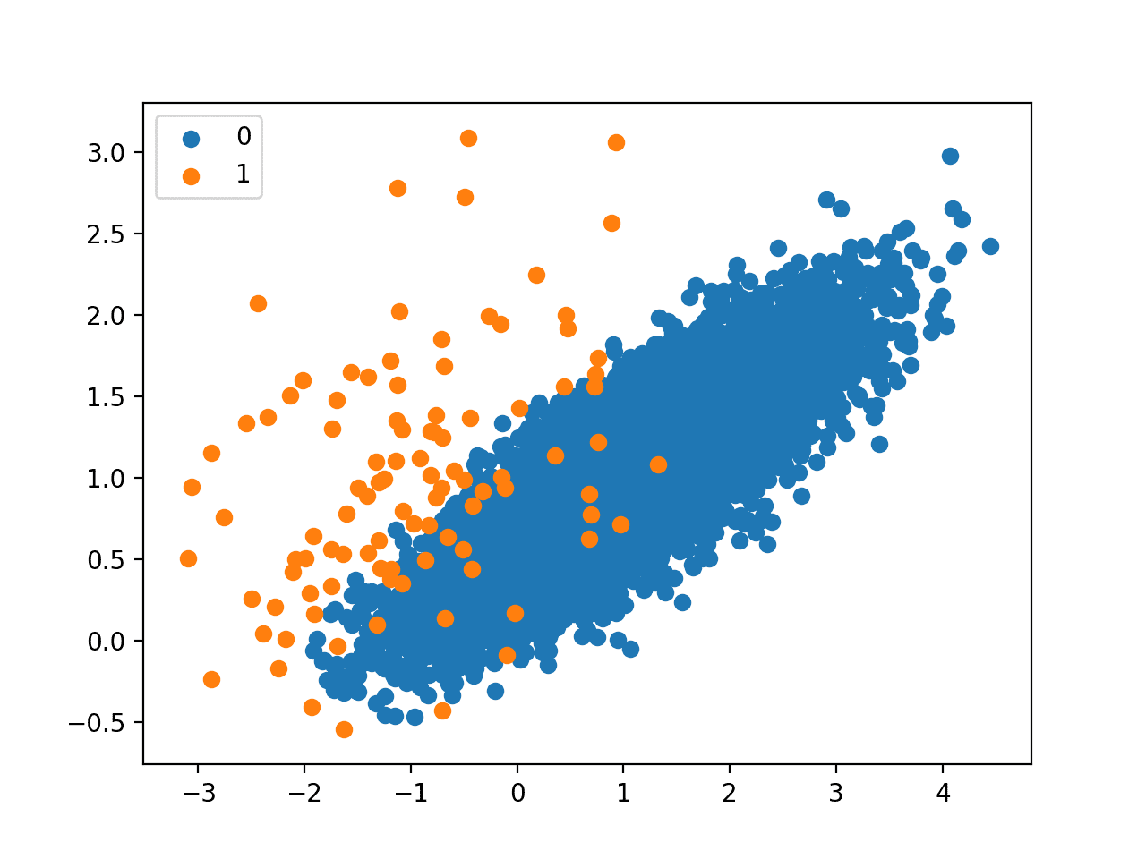
We can then create a scatter plot of the dataset via the scatter() Matplotlib function to understand the spatial relationship of the examples in each class and their imbalance.
|
1 2 3 4 5 6 7 |
... # scatter plot of examples by class label for label, _ in counter.items(): row_ix = where(y == label)[0] pyplot.scatter(X[row_ix, 0], X[row_ix, 1], label=str(label)) pyplot.legend() pyplot.show() |
Tying this together, the complete example of creating an imbalanced classification dataset and plotting the examples is listed below.
|
1 2 3 4 5 6 7 8 9 10 11 12 13 14 15 16 17 |
# Generate and plot a synthetic imbalanced classification dataset from collections import Counter from sklearn.datasets import make_classification from matplotlib import pyplot from numpy import where # define dataset X, y = make_classification(n_samples=10000, n_features=2, n_redundant=0, n_clusters_per_class=1, weights=[0.99], flip_y=0, random_state=1) # summarize class distribution counter = Counter(y) print(counter) # scatter plot of examples by class label for label, _ in counter.items(): row_ix = where(y == label)[0] pyplot.scatter(X[row_ix, 0], X[row_ix, 1], label=str(label)) pyplot.legend() pyplot.show() |
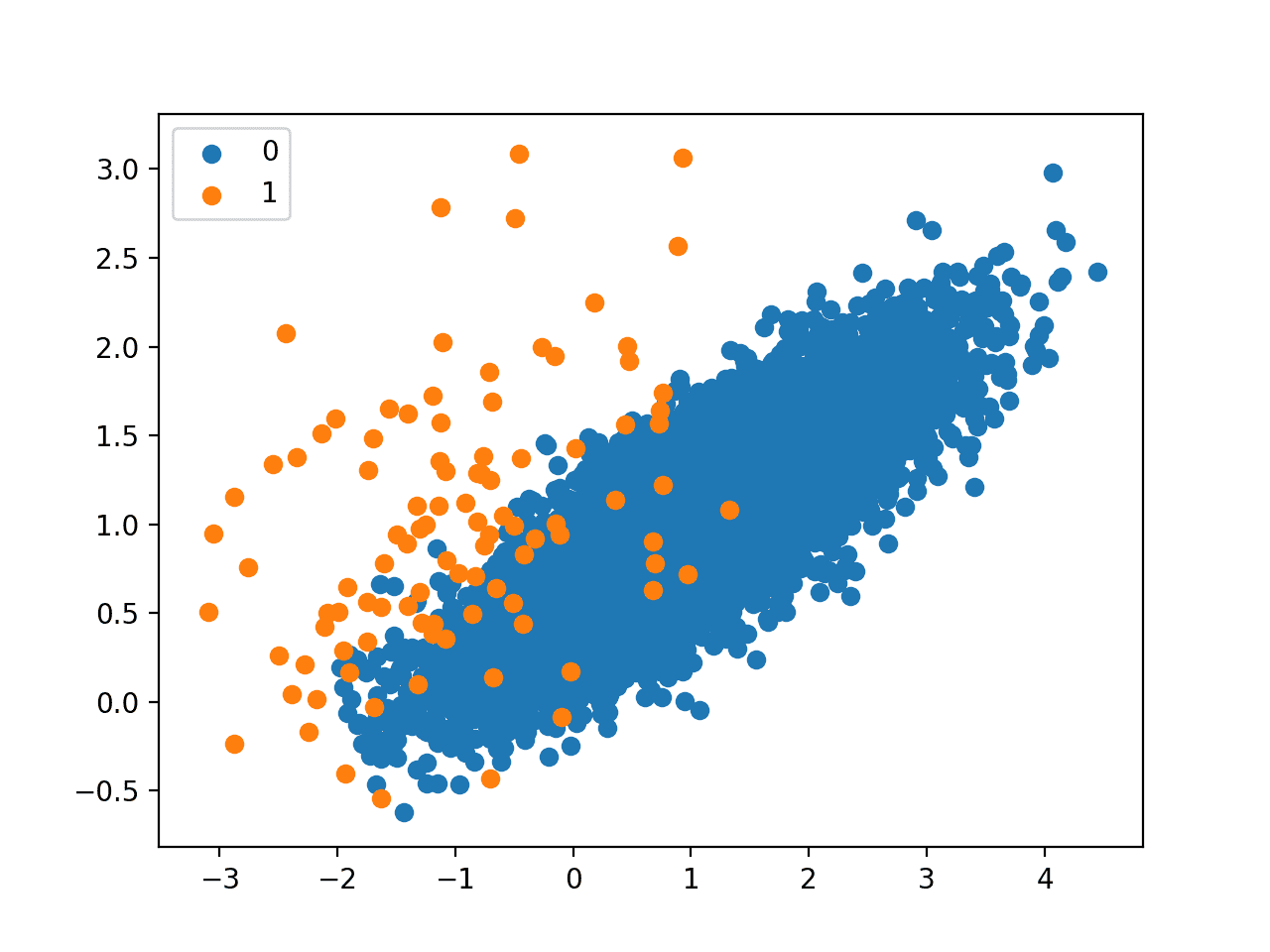
Running the example first summarizes the class distribution, showing an approximate 1:100 class distribution with about 10,000 examples with class 0 and 100 with class 1.
|
1 |
Counter({0: 9900, 1: 100}) |
Next, a scatter plot is created showing all of the examples in the dataset. We can see a large mass of examples for class 0 (blue) and a small number of examples for class 1 (orange). We can also see that the classes overlap with some examples from class 1 clearly within the part of the feature space that belongs to class 0.

Scatter Plot of Imbalanced Classification Dataset
This plot provides the starting point for developing the intuition for the effect that different undersampling techniques have on the majority class.
Next, we can begin to review popular undersampling methods made available via the imbalanced-learn Python library.
There are many different methods to choose from. We will divide them into methods that select what examples from the majority class to keep, methods that select examples to delete, and combinations of both approaches.
Want to Get Started With Imbalance Classification?
Take my free 7-day email crash course now (with sample code).
Click to sign-up and also get a free PDF Ebook version of the course.
Imbalanced-Learn Library
In these examples, we will use the implementations provided by the imbalanced-learn Python library, which can be installed via pip as follows:
|
1 |
sudo pip install imbalanced-learn |
You can confirm that the installation was successful by printing the version of the installed library:
|
1 2 3 |
# check version number import imblearn print(imblearn.__version__) |
Running the example will print the version number of the installed library; for example:
|
1 |
0.5.0 |
Methods that Select Examples to Keep
In this section, we will take a closer look at two methods that choose which examples from the majority class to keep, the near-miss family of methods, and the popular condensed nearest neighbor rule.
Near Miss Undersampling
Near Miss refers to a collection of undersampling methods that select examples based on the distance of majority class examples to minority class examples.
The approaches were proposed by Jianping Zhang and Inderjeet Mani in their 2003 paper titled “KNN Approach to Unbalanced Data Distributions: A Case Study Involving Information Extraction.”
There are three versions of the technique, named NearMiss-1, NearMiss-2, and NearMiss-3.
NearMiss-1 selects examples from the majority class that have the smallest average distance to the three closest examples from the minority class. NearMiss-2 selects examples from the majority class that have the smallest average distance to the three furthest examples from the minority class. NearMiss-3 involves selecting a given number of majority class examples for each example in the minority class that are closest.
Here, distance is determined in feature space using Euclidean distance or similar.
- NearMiss-1: Majority class examples with minimum average distance to three closest minority class examples.
- NearMiss-2: Majority class examples with minimum average distance to three furthest minority class examples.
- NearMiss-3: Majority class examples with minimum distance to each minority class example.
The NearMiss-3 seems desirable, given that it will only keep those majority class examples that are on the decision boundary.
We can implement the Near Miss methods using the NearMiss imbalanced-learn class.
The type of near-miss strategy used is defined by the “version” argument, which by default is set to 1 for NearMiss-1, but can be set to 2 or 3 for the other two methods.
|
1 2 3 |
... # define the undersampling method undersample = NearMiss(version=1) |
By default, the technique will undersample the majority class to have the same number of examples as the minority class, although this can be changed by setting the sampling_strategy argument to a fraction of the minority class.
First, we can demonstrate NearMiss-1 that selects only those majority class examples that have a minimum distance to three minority class instances, defined by the n_neighbors argument.
We would expect clusters of majority class examples around the minority class examples that overlap.
The complete example is listed below.
|
1 2 3 4 5 6 7 8 9 10 11 12 13 14 15 16 17 18 19 20 21 22 23 24 25 |
# Undersample imbalanced dataset with NearMiss-1 from collections import Counter from sklearn.datasets import make_classification from imblearn.under_sampling import NearMiss from matplotlib import pyplot from numpy import where # define dataset X, y = make_classification(n_samples=10000, n_features=2, n_redundant=0, n_clusters_per_class=1, weights=[0.99], flip_y=0, random_state=1) # summarize class distribution counter = Counter(y) print(counter) # define the undersampling method undersample = NearMiss(version=1, n_neighbors=3) # transform the dataset X, y = undersample.fit_resample(X, y) # summarize the new class distribution counter = Counter(y) print(counter) # scatter plot of examples by class label for label, _ in counter.items(): row_ix = where(y == label)[0] pyplot.scatter(X[row_ix, 0], X[row_ix, 1], label=str(label)) pyplot.legend() pyplot.show() |
Running the example undersamples the majority class and creates a scatter plot of the transformed dataset.
We can see that, as expected, only those examples in the majority class that are closest to the minority class examples in the overlapping area were retained.
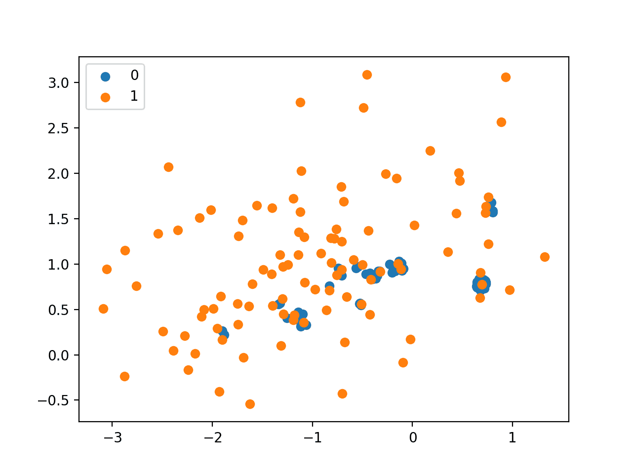
Scatter Plot of Imbalanced Dataset Undersampled with NearMiss-1
Next, we can demonstrate the NearMiss-2 strategy, which is an inverse to NearMiss-1. It selects examples that are closest to the most distant examples from the minority class, defined by the n_neighbors argument.
This is not an intuitive strategy from the description alone.
The complete example is listed below.
|
1 2 3 4 5 6 7 8 9 10 11 12 13 14 15 16 17 18 19 20 21 22 23 24 25 |
# Undersample imbalanced dataset with NearMiss-2 from collections import Counter from sklearn.datasets import make_classification from imblearn.under_sampling import NearMiss from matplotlib import pyplot from numpy import where # define dataset X, y = make_classification(n_samples=10000, n_features=2, n_redundant=0, n_clusters_per_class=1, weights=[0.99], flip_y=0, random_state=1) # summarize class distribution counter = Counter(y) print(counter) # define the undersampling method undersample = NearMiss(version=2, n_neighbors=3) # transform the dataset X, y = undersample.fit_resample(X, y) # summarize the new class distribution counter = Counter(y) print(counter) # scatter plot of examples by class label for label, _ in counter.items(): row_ix = where(y == label)[0] pyplot.scatter(X[row_ix, 0], X[row_ix, 1], label=str(label)) pyplot.legend() pyplot.show() |
Running the example, we can see that the NearMiss-2 selects examples that appear to be in the center of mass for the overlap between the two classes.
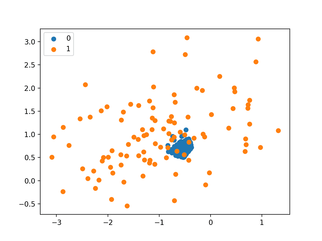
Scatter Plot of Imbalanced Dataset Undersampled With NearMiss-2
Finally, we can try NearMiss-3 that selects the closest examples from the majority class for each minority class.
The n_neighbors_ver3 argument determines the number of examples to select for each minority example, although the desired balancing ratio set via sampling_strategy will filter this so that the desired balance is achieved.
The complete example is listed below.
|
1 2 3 4 5 6 7 8 9 10 11 12 13 14 15 16 17 18 19 20 21 22 23 24 25 |
# Undersample imbalanced dataset with NearMiss-3 from collections import Counter from sklearn.datasets import make_classification from imblearn.under_sampling import NearMiss from matplotlib import pyplot from numpy import where # define dataset X, y = make_classification(n_samples=10000, n_features=2, n_redundant=0, n_clusters_per_class=1, weights=[0.99], flip_y=0, random_state=1) # summarize class distribution counter = Counter(y) print(counter) # define the undersampling method undersample = NearMiss(version=3, n_neighbors_ver3=3) # transform the dataset X, y = undersample.fit_resample(X, y) # summarize the new class distribution counter = Counter(y) print(counter) # scatter plot of examples by class label for label, _ in counter.items(): row_ix = where(y == label)[0] pyplot.scatter(X[row_ix, 0], X[row_ix, 1], label=str(label)) pyplot.legend() pyplot.show() |
As expected, we can see that each example in the minority class that was in the region of overlap with the majority class has up to three neighbors from the majority class.
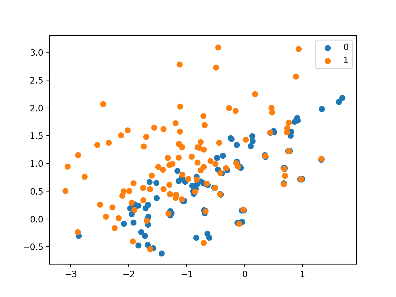
Scatter Plot of Imbalanced Dataset Undersampled With NearMiss-3
Condensed Nearest Neighbor Rule Undersampling
Condensed Nearest Neighbors, or CNN for short, is an undersampling technique that seeks a subset of a collection of samples that results in no loss in model performance, referred to as a minimal consistent set.
… the notion of a consistent subset of a sample set. This is a subset which, when used as a stored reference set for the NN rule, correctly classifies all of the remaining points in the sample set.
— The Condensed Nearest Neighbor Rule (Corresp.), 1968.
It is achieved by enumerating the examples in the dataset and adding them to the “store” only if they cannot be classified correctly by the current contents of the store. This approach was proposed to reduce the memory requirements for the k-Nearest Neighbors (KNN) algorithm by Peter Hart in the 1968 correspondence titled “The Condensed Nearest Neighbor Rule.”
When used for imbalanced classification, the store is comprised of all examples in the minority set and only examples from the majority set that cannot be classified correctly are added incrementally to the store.
We can implement the Condensed Nearest Neighbor for undersampling using the CondensedNearestNeighbour class from the imbalanced-learn library.
During the procedure, the KNN algorithm is used to classify points to determine if they are to be added to the store or not. The k value is set via the n_neighbors argument and defaults to 1.
|
1 2 3 |
... # define the undersampling method undersample = CondensedNearestNeighbour(n_neighbors=1) |
It’s a relatively slow procedure, so small datasets and small k values are preferred.
The complete example of demonstrating the Condensed Nearest Neighbor rule for undersampling is listed below.
|
1 2 3 4 5 6 7 8 9 10 11 12 13 14 15 16 17 18 19 20 21 22 23 24 25 |
# Undersample and plot imbalanced dataset with the Condensed Nearest Neighbor Rule from collections import Counter from sklearn.datasets import make_classification from imblearn.under_sampling import CondensedNearestNeighbour from matplotlib import pyplot from numpy import where # define dataset X, y = make_classification(n_samples=10000, n_features=2, n_redundant=0, n_clusters_per_class=1, weights=[0.99], flip_y=0, random_state=1) # summarize class distribution counter = Counter(y) print(counter) # define the undersampling method undersample = CondensedNearestNeighbour(n_neighbors=1) # transform the dataset X, y = undersample.fit_resample(X, y) # summarize the new class distribution counter = Counter(y) print(counter) # scatter plot of examples by class label for label, _ in counter.items(): row_ix = where(y == label)[0] pyplot.scatter(X[row_ix, 0], X[row_ix, 1], label=str(label)) pyplot.legend() pyplot.show() |
Running the example first reports the skewed distribution of the raw dataset, then the more balanced distribution for the transformed dataset.
We can see that the resulting distribution is about 1:2 minority to majority examples. This highlights that although the sampling_strategy argument seeks to balance the class distribution, the algorithm will continue to add misclassified examples to the store (transformed dataset). This is a desirable property.
|
1 2 |
Counter({0: 9900, 1: 100}) Counter({0: 188, 1: 100}) |
A scatter plot of the resulting dataset is created. We can see that the focus of the algorithm is those examples in the minority class along the decision boundary between the two classes, specifically, those majority examples around the minority class examples.

Scatter Plot of Imbalanced Dataset Undersampled With the Condensed Nearest Neighbor Rule
Methods that Select Examples to Delete
In this section, we will take a closer look at methods that select examples from the majority class to delete, including the popular Tomek Links method and the Edited Nearest Neighbors rule.
Tomek Links for Undersampling
A criticism of the Condensed Nearest Neighbor Rule is that examples are selected randomly, especially initially.
This has the effect of allowing redundant examples into the store and in allowing examples that are internal to the mass of the distribution, rather than on the class boundary, into the store.
The condensed nearest-neighbor (CNN) method chooses samples randomly. This results in a)retention of unnecessary samples and b) occasional retention of internal rather than boundary samples.
— Two modifications of CNN, 1976.
Two modifications to the CNN procedure were proposed by Ivan Tomek in his 1976 paper titled “Two modifications of CNN.” One of the modifications (Method2) is a rule that finds pairs of examples, one from each class; they together have the smallest Euclidean distance to each other in feature space.
This means that in a binary classification problem with classes 0 and 1, a pair would have an example from each class and would be closest neighbors across the dataset.
In words, instances a and b define a Tomek Link if: (i) instance a’s nearest neighbor is b, (ii) instance b’s nearest neighbor is a, and (iii) instances a and b belong to different classes.
— Page 46, Imbalanced Learning: Foundations, Algorithms, and Applications, 2013.
These cross-class pairs are now generally referred to as “Tomek Links” and are valuable as they define the class boundary.
Method 2 has another potentially important property: It finds pairs of boundary points which participate in the formation of the (piecewise-linear) boundary. […] Such methods could use these pairs to generate progressively simpler descriptions of acceptably accurate approximations of the original completely specified boundaries.
— Two modifications of CNN, 1976.
The procedure for finding Tomek Links can be used to locate all cross-class nearest neighbors. If the examples in the minority class are held constant, the procedure can be used to find all of those examples in the majority class that are closest to the minority class, then removed. These would be the ambiguous examples.
From this definition, we see that instances that are in Tomek Links are either boundary instances or noisy instances. This is due to the fact that only boundary instances and noisy instances will have nearest neighbors, which are from the opposite class.
— Page 46, Imbalanced Learning: Foundations, Algorithms, and Applications, 2013.
We can implement Tomek Links method for undersampling using the TomekLinks imbalanced-learn class.
|
1 2 3 |
... # define the undersampling method undersample = TomekLinks() |
The complete example of demonstrating the Tomek Links for undersampling is listed below.
Because the procedure only removes so-named “Tomek Links“, we would not expect the resulting transformed dataset to be balanced, only less ambiguous along the class boundary.
|
1 2 3 4 5 6 7 8 9 10 11 12 13 14 15 16 17 18 19 20 21 22 23 24 25 |
# Undersample and plot imbalanced dataset with Tomek Links from collections import Counter from sklearn.datasets import make_classification from imblearn.under_sampling import TomekLinks from matplotlib import pyplot from numpy import where # define dataset X, y = make_classification(n_samples=10000, n_features=2, n_redundant=0, n_clusters_per_class=1, weights=[0.99], flip_y=0, random_state=1) # summarize class distribution counter = Counter(y) print(counter) # define the undersampling method undersample = TomekLinks() # transform the dataset X, y = undersample.fit_resample(X, y) # summarize the new class distribution counter = Counter(y) print(counter) # scatter plot of examples by class label for label, _ in counter.items(): row_ix = where(y == label)[0] pyplot.scatter(X[row_ix, 0], X[row_ix, 1], label=str(label)) pyplot.legend() pyplot.show() |
Running the example first summarizes the class distribution for the raw dataset, then the transformed dataset.
We can see that only 26 examples from the majority class were removed.
|
1 2 |
Counter({0: 9900, 1: 100}) Counter({0: 9874, 1: 100}) |
The scatter plot of the transformed dataset does not make the minor editing to the majority class obvious.
This highlights that although finding the ambiguous examples on the class boundary is useful, alone, it is not a great undersampling technique. In practice, the Tomek Links procedure is often combined with other methods, such as the Condensed Nearest Neighbor Rule.
The choice to combine Tomek Links and CNN is natural, as Tomek Links can be said to remove borderline and noisy instances, while CNN removes redundant instances.
— Page 46, Imbalanced Learning: Foundations, Algorithms, and Applications, 2013.
Scatter Plot of Imbalanced Dataset Undersampled With the Tomek Links Method
Edited Nearest Neighbors Rule for Undersampling
Another rule for finding ambiguous and noisy examples in a dataset is called Edited Nearest Neighbors, or sometimes ENN for short.
This rule involves using k=3 nearest neighbors to locate those examples in a dataset that are misclassified and that are then removed before a k=1 classification rule is applied. This approach of resampling and classification was proposed by Dennis Wilson in his 1972 paper titled “Asymptotic Properties of Nearest Neighbor Rules Using Edited Data.”
The modified three-nearest neighbor rule which uses the three-nearest neighbor rule to edit the preclassified samples and then uses a single-nearest neighbor rule to make decisions is a particularly attractive rule.
— Asymptotic Properties of Nearest Neighbor Rules Using Edited Data, 1972.
When used as an undersampling procedure, the rule can be applied to each example in the majority class, allowing those examples that are misclassified as belonging to the minority class to be removed, and those correctly classified to remain.
It is also applied to each example in the minority class where those examples that are misclassified have their nearest neighbors from the majority class deleted.
… for each instance a in the dataset, its three nearest neighbors are computed. If a is a majority class instance and is misclassified by its three nearest neighbors, then a is removed from the dataset. Alternatively, if a is a minority class instance and is misclassified by its three nearest neighbors, then the majority class instances among a’s neighbors are removed.
— Page 46, Imbalanced Learning: Foundations, Algorithms, and Applications, 2013.
The Edited Nearest Neighbors rule can be implemented using the EditedNearestNeighbours imbalanced-learn class.
The n_neighbors argument controls the number of neighbors to use in the editing rule, which defaults to three, as in the paper.
|
1 2 3 |
... # define the undersampling method undersample = EditedNearestNeighbours(n_neighbors=3) |
The complete example of demonstrating the ENN rule for undersampling is listed below.
Like Tomek Links, the procedure only removes noisy and ambiguous points along the class boundary. As such, we would not expect the resulting transformed dataset to be balanced.
|
1 2 3 4 5 6 7 8 9 10 11 12 13 14 15 16 17 18 19 20 21 22 23 24 25 |
# Undersample and plot imbalanced dataset with the Edited Nearest Neighbor rule from collections import Counter from sklearn.datasets import make_classification from imblearn.under_sampling import EditedNearestNeighbours from matplotlib import pyplot from numpy import where # define dataset X, y = make_classification(n_samples=10000, n_features=2, n_redundant=0, n_clusters_per_class=1, weights=[0.99], flip_y=0, random_state=1) # summarize class distribution counter = Counter(y) print(counter) # define the undersampling method undersample = EditedNearestNeighbours(n_neighbors=3) # transform the dataset X, y = undersample.fit_resample(X, y) # summarize the new class distribution counter = Counter(y) print(counter) # scatter plot of examples by class label for label, _ in counter.items(): row_ix = where(y == label)[0] pyplot.scatter(X[row_ix, 0], X[row_ix, 1], label=str(label)) pyplot.legend() pyplot.show() |
Running the example first summarizes the class distribution for the raw dataset, then the transformed dataset.
We can see that only 94 examples from the majority class were removed.
|
1 2 |
Counter({0: 9900, 1: 100}) Counter({0: 9806, 1: 100}) |
Given the small amount of undersampling performed, the change to the mass of majority examples is not obvious from the plot.
Also, like Tomek Links, the Edited Nearest Neighbor Rule gives best results when combined with another undersampling method.
Scatter Plot of Imbalanced Dataset Undersampled With the Edited Nearest Neighbor Rule
Ivan Tomek, developer of Tomek Links, explored extensions of the Edited Nearest Neighbor Rule in his 1976 paper titled “An Experiment with the Edited Nearest-Neighbor Rule.”
Among his experiments was a repeated ENN method that invoked the continued editing of the dataset using the ENN rule for a fixed number of iterations, referred to as “unlimited editing.”
… unlimited repetition of Wilson’s editing (in fact, editing is always stopped after a finite number of steps because after a certain number of repetitions the design set becomes immune to further elimination)
— An Experiment with the Edited Nearest-Neighbor Rule, 1976.
He also describes a method referred to as “all k-NN” that removes all examples from the dataset that were classified incorrectly.
Both of these additional editing procedures are also available via the imbalanced-learn library via the RepeatedEditedNearestNeighbours and AllKNN classes.
Combinations of Keep and Delete Methods
In this section, we will take a closer look at techniques that combine the techniques we have already looked at to both keep and delete examples from the majority class, such as One-Sided Selection and the Neighborhood Cleaning Rule.
One-Sided Selection for Undersampling
One-Sided Selection, or OSS for short, is an undersampling technique that combines Tomek Links and the Condensed Nearest Neighbor (CNN) Rule.
Specifically, Tomek Links are ambiguous points on the class boundary and are identified and removed in the majority class. The CNN method is then used to remove redundant examples from the majority class that are far from the decision boundary.
OSS is an undersampling method resulting from the application of Tomek links followed by the application of US-CNN. Tomek links are used as an undersampling method and removes noisy and borderline majority class examples. […] US-CNN aims to remove examples from the majority class that are distant from the decision border.
— Page 84, Learning from Imbalanced Data Sets, 2018.
This combination of methods was proposed by Miroslav Kubat and Stan Matwin in their 1997 paper titled “Addressing The Curse Of Imbalanced Training Sets: One-sided Selection.”
The CNN procedure occurs in one-step and involves first adding all minority class examples to the store and some number of majority class examples (e.g. 1), then classifying all remaining majority class examples with KNN (k=1) and adding those that are misclassified to the store.
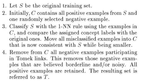
Overview of the One-Sided Selection for Undersampling Procedure
Taken from Addressing The Curse Of Imbalanced Training Sets: One-sided Selection.
We can implement the OSS undersampling strategy via the OneSidedSelection imbalanced-learn class.
The number of seed examples can be set with n_seeds_S and defaults to 1 and the k for KNN can be set via the n_neighbors argument and defaults to 1.
Given that the CNN procedure occurs in one block, it is more useful to have a larger seed sample of the majority class in order to effectively remove redundant examples. In this case, we will use a value of 200.
|
1 2 3 |
... # define the undersampling method undersample = OneSidedSelection(n_neighbors=1, n_seeds_S=200) |
The complete example of applying OSS on the binary classification problem is listed below.
We might expect a large number of redundant examples from the majority class to be removed from the interior of the distribution (e.g. away from the class boundary).
|
1 2 3 4 5 6 7 8 9 10 11 12 13 14 15 16 17 18 19 20 21 22 23 24 25 |
# Undersample and plot imbalanced dataset with One-Sided Selection from collections import Counter from sklearn.datasets import make_classification from imblearn.under_sampling import OneSidedSelection from matplotlib import pyplot from numpy import where # define dataset X, y = make_classification(n_samples=10000, n_features=2, n_redundant=0, n_clusters_per_class=1, weights=[0.99], flip_y=0, random_state=1) # summarize class distribution counter = Counter(y) print(counter) # define the undersampling method undersample = OneSidedSelection(n_neighbors=1, n_seeds_S=200) # transform the dataset X, y = undersample.fit_resample(X, y) # summarize the new class distribution counter = Counter(y) print(counter) # scatter plot of examples by class label for label, _ in counter.items(): row_ix = where(y == label)[0] pyplot.scatter(X[row_ix, 0], X[row_ix, 1], label=str(label)) pyplot.legend() pyplot.show() |
Running the example first reports the class distribution in the raw dataset, then the transformed dataset.
We can see that a large number of examples from the majority class were removed, consisting of both redundant examples (removed via CNN) and ambiguous examples (removed via Tomek Links). The ratio for this dataset is now around 1:10., down from 1:100.
|
1 2 |
Counter({0: 9900, 1: 100}) Counter({0: 940, 1: 100}) |
A scatter plot of the transformed dataset is created showing that most of the majority class examples left belong are around the class boundary and the overlapping examples from the minority class.
It might be interesting to explore larger seed samples from the majority class and different values of k used in the one-step CNN procedure.
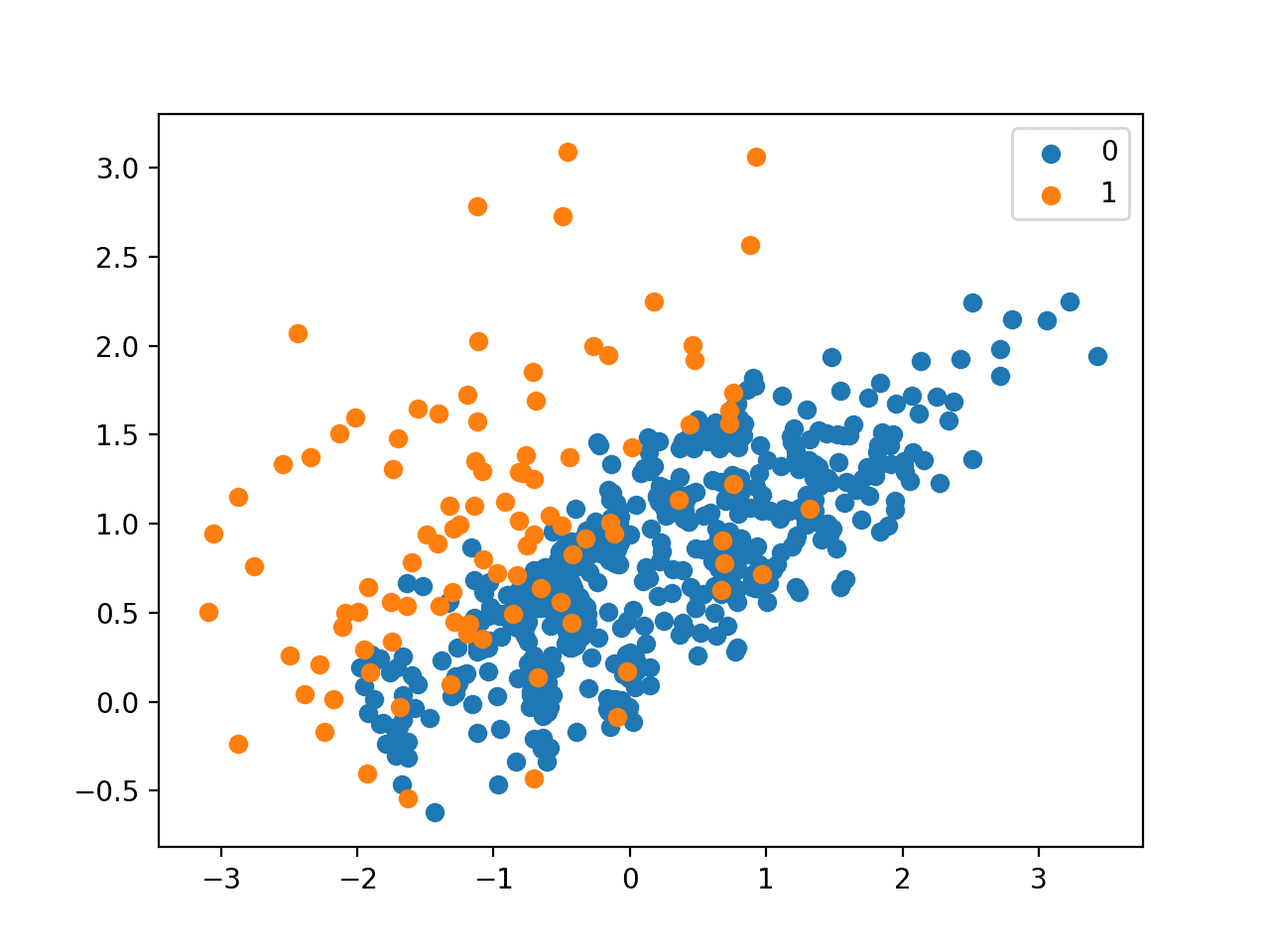
Scatter Plot of Imbalanced Dataset Undersampled With One-Sided Selection
Neighborhood Cleaning Rule for Undersampling
The Neighborhood Cleaning Rule, or NCR for short, is an undersampling technique that combines both the Condensed Nearest Neighbor (CNN) Rule to remove redundant examples and the Edited Nearest Neighbors (ENN) Rule to remove noisy or ambiguous examples.
Like One-Sided Selection (OSS), the CSS method is applied in a one-step manner, then the examples that are misclassified according to a KNN classifier are removed, as per the ENN rule. Unlike OSS, less of the redundant examples are removed and more attention is placed on “cleaning” those examples that are retained.
The reason for this is to focus less on improving the balance of the class distribution and more on the quality (unambiguity) of the examples that are retained in the majority class.
… the quality of classification results does not necessarily depend on the size of the class. Therefore, we should consider, besides the class distribution, other characteristics of data, such as noise, that may hamper classification.
— Improving Identification of Difficult Small Classes by Balancing Class Distribution, 2001.
This approach was proposed by Jorma Laurikkala in her 2001 paper titled “Improving Identification of Difficult Small Classes by Balancing Class Distribution.”
The approach involves first selecting all examples from the minority class. Then all of the ambiguous examples in the majority class are identified using the ENN rule and removed. Finally, a one-step version of CNN is used where those remaining examples in the majority class that are misclassified against the store are removed, but only if the number of examples in the majority class is larger than half the size of the minority class.
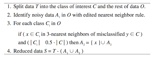
Summary of the Neighborhood Cleaning Rule Algorithm.
Taken from Improving Identification of Difficult Small Classes by Balancing Class Distribution.
This technique can be implemented using the NeighbourhoodCleaningRule imbalanced-learn class. The number of neighbors used in the ENN and CNN steps can be specified via the n_neighbors argument that defaults to three. The threshold_cleaning controls whether or not the CNN is applied to a given class, which might be useful if there are multiple minority classes with similar sizes. This is kept at 0.5.
The complete example of applying NCR on the binary classification problem is listed below.
Given the focus on data cleaning over removing redundant examples, we would expect only a modest reduction in the number of examples in the majority class.
|
1 2 3 4 5 6 7 8 9 10 11 12 13 14 15 16 17 18 19 20 21 22 23 24 25 |
# Undersample and plot imbalanced dataset with the neighborhood cleaning rule from collections import Counter from sklearn.datasets import make_classification from imblearn.under_sampling import NeighbourhoodCleaningRule from matplotlib import pyplot from numpy import where # define dataset X, y = make_classification(n_samples=10000, n_features=2, n_redundant=0, n_clusters_per_class=1, weights=[0.99], flip_y=0, random_state=1) # summarize class distribution counter = Counter(y) print(counter) # define the undersampling method undersample = NeighbourhoodCleaningRule(n_neighbors=3, threshold_cleaning=0.5) # transform the dataset X, y = undersample.fit_resample(X, y) # summarize the new class distribution counter = Counter(y) print(counter) # scatter plot of examples by class label for label, _ in counter.items(): row_ix = where(y == label)[0] pyplot.scatter(X[row_ix, 0], X[row_ix, 1], label=str(label)) pyplot.legend() pyplot.show() |
Running the example first reports the class distribution in the raw dataset, then the transformed dataset.
We can see that only 114 examples from the majority class were removed.
|
1 2 |
Counter({0: 9900, 1: 100}) Counter({0: 9786, 1: 100}) |
Given the limited and focused amount of undersampling performed, the change to the mass of majority examples is not obvious from the scatter plot that is created.

Scatter Plot of Imbalanced Dataset Undersampled With the Neighborhood Cleaning Rule
Further Reading
This section provides more resources on the topic if you are looking to go deeper.
Papers
- kNN Approach To Unbalanced Data Distributions: A Case Study Involving Information Extraction, 2003.
- The Condensed Nearest Neighbor Rule (Corresp.), 1968
- Two modifications of CNN, 1976.
- Addressing The Curse Of Imbalanced Training Sets: One-sided Selection, 1997.
- Asymptotic Properties of Nearest Neighbor Rules Using Edited Data, 1972.
- An Experiment with the Edited Nearest-Neighbor Rule, 1976.
- Improving Identification of Difficult Small Classes by Balancing Class Distribution, 2001.
Books
- Learning from Imbalanced Data Sets, 2018.
- Imbalanced Learning: Foundations, Algorithms, and Applications, 2013.
API
- Under-sampling, Imbalanced-Learn User Guide.
- imblearn.under_sampling.NearMiss API
- imblearn.under_sampling.CondensedNearestNeighbour API
- imblearn.under_sampling.TomekLinks API
- imblearn.under_sampling.OneSidedSelection API
- imblearn.under_sampling.EditedNearestNeighbours API.
- imblearn.under_sampling.NeighbourhoodCleaningRule API
Articles
Summary
In this tutorial, you discovered undersampling methods for imbalanced classification.
Specifically, you learned:
- How to use the Near-Miss and Condensed Nearest Neighbor Rule methods that select examples to keep from the majority class.
- How to use Tomek Links and the Edited Nearest Neighbors Rule methods that select examples to delete from the majority class.
- How to use One-Sided Selection and the Neighborhood Cleaning Rule that combine methods for choosing examples to keep and delete from the majority class.
Do you have any questions?
Ask your questions in the comments below and I will do my best to answer.
Get a Handle on Imbalanced Classification!

Develop Imbalanced Learning Models in Minutes
...with just a few lines of python code
Discover how in my new Ebook:
Imbalanced Classification with Python
It provides self-study tutorials and end-to-end projects on:
Performance Metrics, Undersampling Methods, SMOTE, Threshold Moving, Probability Calibration, Cost-Sensitive Algorithms
and much more...


")


Thanks for another great article..
Please let me know.. how to get your books in India?
You can purchase the books directly from the website from any country:
https://machinelearningmastery.com/products/
Hello Jason,
when I use GridSearchCV is there any rules of thumb to select which hyperparameter
to choose in order to have better performances of the model.
Thanks,
Marco
Yes, perhaps ranges for hyperparameters that have worked well in the past on related problems.
Hello Jason,
I’ve taken a look on the web and I’ve seen most common hyperparameters for RandomForestClassifier, XGBClassifier and GradientBoostingClassifier are
n_estimators (question: Are they numbers of trees?)
max_depth (question: Is it the depth of eache tree?)
(Up to you) any other valuable hyperparameter to take a look at?
I had a look also at the catboost. Performance are more or less the same in comparison with XGBClassifier.
How to improve the performance of them? Is it a matter of hyperparameters tuning?
Thanks
Marco
Yes in both cases.
Yes, there are more, see this:
https://machinelearningmastery.com/hyperparameters-for-classification-machine-learning-algorithms/
Very nice guide! Really appreciate the reproducible examples.
Thanks!
Hey Jason, your website is a wonderful resource. Could you share any intuition on which undersampling is the most efficient one? I have a slightly imbalanced dataset with over 2 million entries…
Thanks.
Random is computationally efficient. Others, well, it might be best to benchmark them rather than trying to estimate their complexity.
Good morning!
While dealing with imbalanced classification problems such idea came to my mind: would it make sense to remove “duplicate” points from the majority class (defining them as neighbors having distance lower than some small threshold)? Does having such almost identical instances bring any value to predictive models? Did you have some experience with similar approach?
Regards!
Duplicates should probably be removed as part of data cleaning:
https://machinelearningmastery.com/basic-data-cleaning-for-machine-learning/
How can we change distance from Euclidean to others like Jaccard for NearMiss method?
Great question!
Off hand, I don’t think the imbalanced-learn library supports arbitrary distance functions. You may need to extend the library with custom code.
Hello Jason,
I am building a LSTM classification model. The data has an imbalanced multi class, total 9 classes. Majority class has 59287 instances and least minority class has 2442 instances. In this case to handle imbalance class problem which is good approach, oversampling or undersampling or cost – sensitive method.
Perhaps try cost-sensitive learning instead.
Hello Jason,
Thank you for your blog. It is very instructive.
Based on your comment, I have read this paper [1] and I would like to understand how/why you came up with this suggestion.
Moreover, I was wondering which of One-Sided Selection (OSS) and Neighbourhood Cleaning Rule (NCL) is more efficient. To this interrogation, I think it may depend on the datasets. A practical experiment could provide more information about their performances. I wonder your opinion on it.
[1] 10.1109/IJCNN.2010.5596486
Thank you very much
You’re welcome.
Perhaps try both on your dataset and use the one that results in the best performance.
Hello, i just found a typo mistake that changes the logic of understanding. In the above document where we explain the implementaiton of NearMiss-1
”First, we can demonstrate NearMiss-1 that selects only those majority class examples that have a minimum distance to three majority class instances, defined by the n_neighbors argument.”, shouldnt it be three minority class and not three majority class ?
Thanks
Thanks, fixed.
Hello, Your website is really helpful for me to clear my doubts. Though I have one more doubt. I want to do over sampling using SMOTE. Let’s say there are missing data in a dataset. Now if I use SimpleImputer() and pass it through pipeline, SimpleImputer will try to replace Nan values with mean by default. SMOTE uses KNN approach.
If I replace Nan values with mean before train_test_split and train a model, then there will be information leakage. What should I do in this situation?
Thanks.
Yes, train impute on the training set, apply to train and test sets. Then apply smote to train set.
If you use a pipeline with cv, this will be automatic.
Hi Jason, thank you for the great examples.
I’m struggling to change the colour of the points on the scatterplot. Do you have any tips on how to change it?
I tried the color option but it changes all the points to one colour.
It may be best to check the matplotlib API and examples.
Hello Jason, thank you for the article, it’s been very helpful. But I have a question.
I applied the Near Miss 3 method for a dataset that has 24 columns & 42350 rows, and there is a huge imbalance between data in some columns, while the others have balanced data. My problem is after I implemented Near Miss 3 and fixed imbalanced data, some columns have 30 remained values in them while the others have 8012. This creates a massive gap, a massive amount of Na values when I tried to merge them. I replaced Na values with the mean of each column, most frequent values of each column or std of each column by sklearns SimpleImputer. But this time the values that are replaced with Na’s creates more imbalanced data. In other words, I am creating the other and more imbalanced dataset when I tried to balance my dataset.
I’ve decided to solve this problem by applying less sensitive M.L. algorithms like tree-based ones or evaluating my models metric by F1 Score or ROC AUC Score. It is working, but I want to balance my imbalanced data to apply other algorithms. By the way, my problem is a binary classification problem.
Is there any way to imbalance my dataset with Near Miss 3 or other methods that you mentioned in this article without creating more imbalanced data, or moving on with tree-based models or F1 & ROC AUC Score?
Perhaps you can adjust the configuration of near miss, e.g. experiment and review the results?
Perhaps you can try an alternate technique and compare the results?
What kind of configurations that we’re talking about?
Which alternative technique could be comparable in my case, because all of them will remove data and my problem will remain the same.
Could you be more specific?
Perhaps try a suite of undersampling techniques (such as those in the above tutorial) and discover what works well or best for your specific dataset and chosen model.
Hello again Jason, I tried all of the undersampling techniques in the above tutorial but my problem still continues. Here you can find my trials and their outcomes: https://github.com/talfik2/undersampling_problem
I also added my dataset with my code so that you can examine it better.
Sorry to hear that.
I don’t have the capacity to review your code, I hope you can understand.
Hello Jason..! It’s a really good and informative article. What is the best method in near-miss? Is it version 3?
Thanks!
Perhaps evaluate each version on your dataset and compare the results.
Thank you!
Hi Jason.
Thanks for this article! Much appreciated.
Which method would you recommend as generally the best to overcome the imbalanced classification problem?
Especially for the medical field.
For example, my dataset has 9,354 rows of class = 0, and 136 rows for class = 1
I tried shuffling the dataset, created separate data frames for the classes, respectively, with the one for class = 0, I got a random set of 136 rows. Then, concatenated both data frames.
I did the above on the main dataset (no splits between train and test) – is this fine?
However, even with parameter tuning, the average results are as follows:
accuracy = 0.5474, AUC = 0, recall = 0.1511, precision = 0.600, F1 = 0.2333
I’ve used pycaret for the above, to try to quickly get results out.
Would you suggest I try any of the undersampling methods you’ve mentioned in this article?
I also was wondering if I should instead try a pre-trained model?
Please help. Much and truly appreciated, in advance.
Yes, try oversampling/undersampling. I am not sure it works, however, because every problem can be different.
I’m concerned about comparing the results of different approaches to deal with imbalanced datasets.
I have tried random undersampling/oversampling, imblearn under/oversampling, and many others, including some of the techniques, described here.
My question is: Should I use the test sample coming from the ORIGINAL dataset or from the modified balanced dataset? Almost every method gives good results when testing with the balanced dataset, but almost none gives a good recall or precision metrics when tested on the original test sample and it makes not much sense to me testing the model other than in the original dataset.
Thank you