This tutorial presents two essential concepts in data science and automated learning. One is the machine learning pipeline, and the second is its optimization. These two principles are the key to implementing any successful intelligent system based on machine learning.
A machine learning pipeline can be created by putting together a sequence of steps involved in training a machine learning model. It can be used to automate a machine learning workflow. The pipeline can involve pre-processing, feature selection, classification/regression, and post-processing. More complex applications may need to fit in other necessary steps within this pipeline.
By optimization, we mean tuning the model for the best performance. The success of any learning model rests on the selection of the best parameters that give the best possible results. Optimization can be looked at in terms of a search algorithm, which walks through a space of parameters and hunts down the best out of them.
After completing this tutorial, you should:
- Appreciate the significance of a pipeline and its optimization.
- Be able to set up a machine learning pipeline.
- Be able to optimize the pipeline.
- Know techniques to analyze the results of optimization.
Kick-start your project with my new book Optimization for Machine Learning, including step-by-step tutorials and the Python source code files for all examples.
The tutorial is simple and easy to follow. It should not take you too long to go through it. So enjoy!Tutorial Overview
This tutorial will show you how to
- Set up a pipeline using the Pipeline object from sklearn.pipeline.
- Perform a grid search for the best parameters using GridSearchCV() from sklearn.model_selection
- Analyze the results from the GridSearchCV() and visualize them
Before we demonstrate all the above, let’s write the import section:
|
1 2 3 4 5 6 7 8 9 10 11 12 |
from pandas import read_csv # For dataframes from pandas import DataFrame # For dataframes from numpy import ravel # For matrices import matplotlib.pyplot as plt # For plotting data import seaborn as sns # For plotting data from sklearn.model_selection import train_test_split # For train/test splits from sklearn.neighbors import KNeighborsClassifier # The k-nearest neighbor classifier from sklearn.feature_selection import VarianceThreshold # Feature selector from sklearn.pipeline import Pipeline # For setting up pipeline # Various pre-processing steps from sklearn.preprocessing import Normalizer, StandardScaler, MinMaxScaler, PowerTransformer, MaxAbsScaler, LabelEncoder from sklearn.model_selection import GridSearchCV # For optimization |
The Dataset
We’ll use the Ecoli Dataset from the UCI Machine Learning Repository to demonstrate all the concepts of this tutorial. This dataset is maintained by Kenta Nakai. Let’s first load the Ecoli dataset in a Pandas DataFrame and view the first few rows.
|
1 2 3 4 5 6 7 |
# Read ecoli dataset from the UCI ML Repository and store in # dataframe df df = read_csv( 'https://archive.ics.uci.edu/ml/machine-learning-databases/ecoli/ecoli.data', sep = '\s+', header=None) print(df.head()) |
Running the example you should see the following:
|
1 2 3 4 5 6 |
0 1 2 3 4 5 6 7 8 0 AAT_ECOLI 0.49 0.29 0.48 0.5 0.56 0.24 0.35 cp 1 ACEA_ECOLI 0.07 0.40 0.48 0.5 0.54 0.35 0.44 cp 2 ACEK_ECOLI 0.56 0.40 0.48 0.5 0.49 0.37 0.46 cp 3 ACKA_ECOLI 0.59 0.49 0.48 0.5 0.52 0.45 0.36 cp 4 ADI_ECOLI 0.23 0.32 0.48 0.5 0.55 0.25 0.35 cp |
We’ll ignore the first column, which specifies the sequence name. The last column is the class label. Let’s separate the features from the class label and split the dataset into 2/3 training instances and 1/3 test examples.
|
1 2 3 4 5 6 7 8 9 10 11 12 13 14 15 16 17 18 19 |
... # The data matrix X X = df.iloc[:,1:-1] # The labels y = (df.iloc[:,-1:]) # Encode the labels into unique integers encoder = LabelEncoder() y = encoder.fit_transform(ravel(y)) # Split the data into test and train X_train, X_test, y_train, y_test = train_test_split( X, y, test_size=1/3, random_state=0) print(X_train.shape) print(X_test.shape) |
Running the example you should see the following:
|
1 2 |
(224, 7) (112, 7) |
Great! Now we have 224 samples in the training set and 112 samples in the test set. We have chosen a small dataset so that we can focus on the concepts, rather than the data itself.
For this tutorial, we have chosen the k-nearest neighbor classifier to perform the classification of this dataset.
Want to Get Started With Optimization Algorithms?
Take my free 7-day email crash course now (with sample code).
Click to sign-up and also get a free PDF Ebook version of the course.
A Classifier Without a Pipeline and Optimization
First, let’s just check how the k-nearest neighbor performs on the training and test sets. This would give us a baseline for performance.
|
1 2 3 4 |
... knn = KNeighborsClassifier().fit(X_train, y_train) print('Training set score: ' + str(knn.score(X_train,y_train))) print('Test set score: ' + str(knn.score(X_test,y_test))) |
Running the example you should see the following:
|
1 2 |
Training set score: 0.9017857142857143 Test set score: 0.8482142857142857 |
We should keep in mind that the true judge of a classifier’s performance is the test set score and not the training set score. The test set score reflects the generalization ability of a classifier.
Setting Up a Machine Learning Pipeline
For this tutorial, we’ll set up a very basic pipeline that consists of the following sequence:
- Scaler: For pre-processing data, i.e., transform the data to zero mean and unit variance using the StandardScaler().
- Feature selector: Use VarianceThreshold() for discarding features whose variance is less than a certain defined threshold.
- Classifier: KNeighborsClassifier(), which implements the k-nearest neighbor classifier and selects the class of the majority k points, which are closest to the test example.
|
1 2 3 4 5 6 |
... pipe = Pipeline([ ('scaler', StandardScaler()), ('selector', VarianceThreshold()), ('classifier', KNeighborsClassifier()) ]) |
The pipe object is simple to understand. It says, scale first, select features second and classify in the end. Let’s call fit() method of the pipe object on our training data and get the training and test scores.
|
1 2 3 4 5 |
... pipe.fit(X_train, y_train) print('Training set score: ' + str(pipe.score(X_train,y_train))) print('Test set score: ' + str(pipe.score(X_test,y_test))) |
Running the example you should see the following:
|
1 2 |
Training set score: 0.8794642857142857 Test set score: 0.8392857142857143 |
So it looks like the performance of this pipeline is worse than the single classifier performance on raw data. Not only did we add extra processing, but it was all in vain. Don’t despair, the real benefit of the pipeline comes from its tuning. The next section explains how to do that.
Optimizing and Tuning the Pipeline
In the code below, we’ll show the following:
- We can search for the best scalers. Instead of just the StandardScaler(), we can try MinMaxScaler(), Normalizer() and MaxAbsScaler().
- We can search for the best variance threshold to use in the selector, i.e., VarianceThreshold().
- We can search for the best value of k for the KNeighborsClassifier().
The parameters variable below is a dictionary that specifies the key:value pairs. Note the key must be written, with a double underscore __ separating the module name that we selected in the Pipeline() and its parameter. Note the following:
- The scaler has no double underscore, as we have specified a list of objects there.
- We would search for the best threshold for the selector, i.e., VarianceThreshold(). Hence we have specified a list of values [0, 0.0001, 0.001, 0.5] to choose from.
- Different values are specified for the n_neighbors, p and leaf_size parameters of the KNeighborsClassifier().
|
1 2 3 4 5 6 7 8 |
... parameters = {'scaler': [StandardScaler(), MinMaxScaler(), Normalizer(), MaxAbsScaler()], 'selector__threshold': [0, 0.001, 0.01], 'classifier__n_neighbors': [1, 3, 5, 7, 10], 'classifier__p': [1, 2], 'classifier__leaf_size': [1, 5, 10, 15] } |
The pipe along with the above list of parameters are then passed to a GridSearchCV() object, that searches the parameters space for the best set of parameters as shown below:
|
1 2 3 4 5 |
... grid = GridSearchCV(pipe, parameters, cv=2).fit(X_train, y_train) print('Training set score: ' + str(grid.score(X_train, y_train))) print('Test set score: ' + str(grid.score(X_test, y_test))) |
Running the example you should see the following:
|
1 2 |
Training set score: 0.8928571428571429 Test set score: 0.8571428571428571 |
By tuning the pipeline, we achieved quite an improvement over a simple classifier and a non-optimized pipeline. It is important to analyze the results of the optimization process.
Don’t worry too much about the warning that you get by running the code above. It is generated because we have very few training samples and the cross-validation object does not have enough samples for a class for one of its folds.
Analyzing the Results
Let’s look at the tuned grid object and gain an understanding of the GridSearchCV() object.
The object is so named because it sets up a multi-dimensional grid, with each corner representing a combination of parameters to try. This defines a parameter space. As an example if we have three values of n_neighbors, i.e., {1,3,5}, two values of leaf_size, i.e., {1,5} and two values of threshold, i.e., {0,0.0001}, then we have a 3D grid with 3x2x2=12 corners. Each corner represents a different combination.
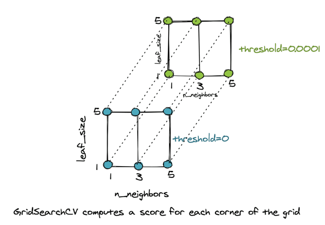
GridSearchCV Computes a Score For Each Corner of the Grid
For each corner of the above grid, the GridSearchCV() object computes the mean cross-validation score on the unseen examples and selects the corner/combination of parameters that give the best result. The code below shows how to access the best parameters of the grid and the best pipeline for our task.
|
1 2 3 4 5 6 7 |
... # Access the best set of parameters best_params = grid.best_params_ print(best_params) # Stores the optimum model in best_pipe best_pipe = grid.best_estimator_ print(best_pipe) |
Running the example you should see the following:
|
1 2 3 4 5 |
{'classifier__leaf_size': 1, 'classifier__n_neighbors': 7, 'classifier__p': 2, 'scaler': StandardScaler(), 'selector__threshold': 0} Pipeline(steps=[('scaler', StandardScaler()), ('selector', VarianceThreshold(threshold=0)), ('classifier', KNeighborsClassifier(leaf_size=1, n_neighbors=7))]) |
Another useful technique for analyzing the results is to construct a DataFrame from the grid.cv_results_. Let’s view the columns of this data frame.
|
1 2 3 |
... result_df = DataFrame.from_dict(grid.cv_results_, orient='columns') print(result_df.columns) |
Running the example you should see the following:
|
1 2 3 4 5 6 |
Index(['mean_fit_time', 'std_fit_time', 'mean_score_time', 'std_score_time', 'param_classifier__leaf_size', 'param_classifier__n_neighbors', 'param_classifier__p', 'param_scaler', 'param_selector__threshold', 'params', 'split0_test_score', 'split1_test_score', 'mean_test_score', 'std_test_score', 'rank_test_score'], dtype='object') |
This DataFrame is very valuable as it shows us the scores for different parameters. The column with the mean_test_score is the average of the scores on the test set for all the folds during cross-validation. The DataFrame may be too big to visualize manually, hence, it is always a good idea to plot the results. Let’s see how n_neighbors affect the performance for different scalers and for different values of p.
|
1 2 3 4 5 6 7 8 |
... sns.relplot(data=result_df, kind='line', x='param_classifier__n_neighbors', y='mean_test_score', hue='param_scaler', col='param_classifier__p') plt.show() |
Running the example you should see the following:
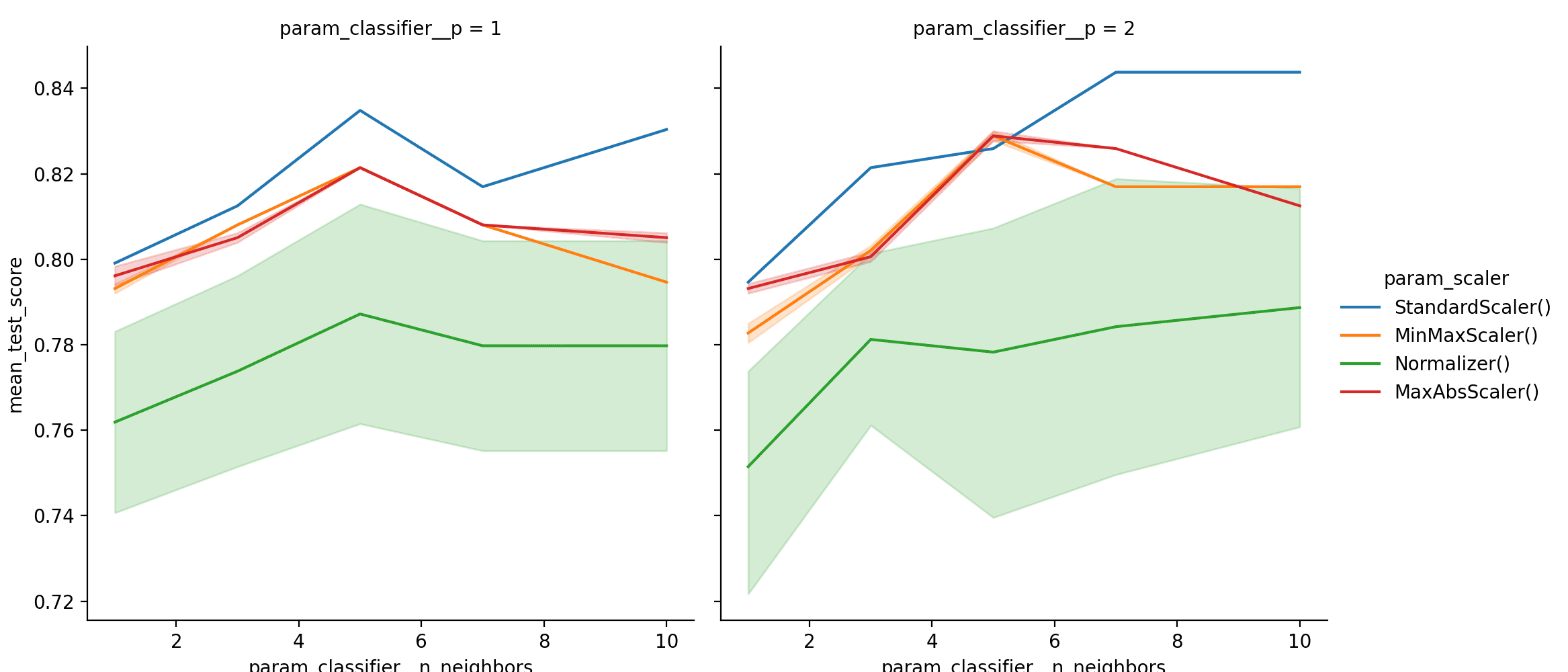
Line Plot of Pipeline GridSearchCV Results
The plots clearly show that using StandardScaler(), with n_neighbors=7 and p=2, gives the best result. Let’s make one more set of plots with leaf_size.
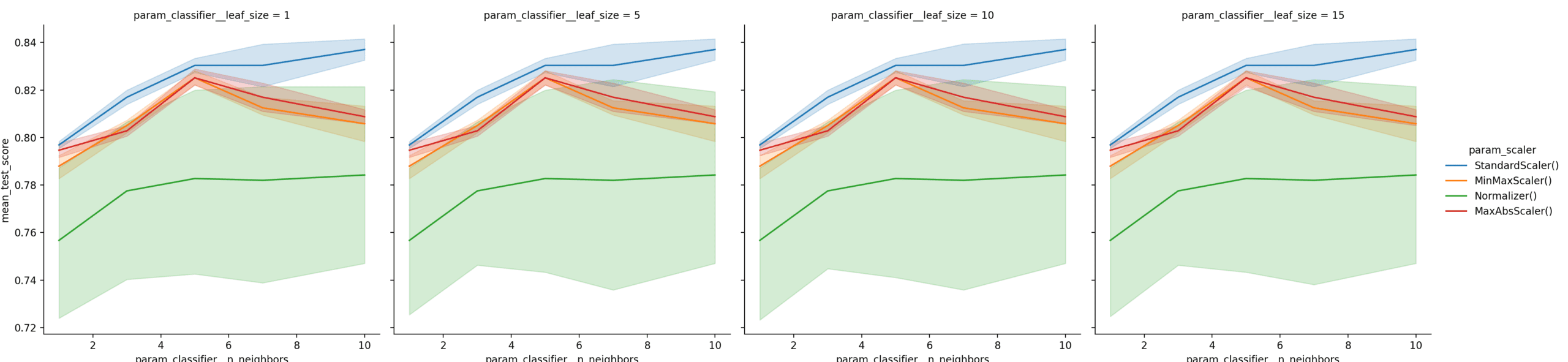
|
1 2 3 4 5 6 7 8 |
... sns.relplot(data=result_df, kind='line', x='param_classifier__n_neighbors', y='mean_test_score', hue='param_scaler', col='param_classifier__leaf_size') plt.show() |
Running the example you should see the following:
Complete Example
Tying this all together, the complete code example is listed below.
|
1 2 3 4 5 6 7 8 9 10 11 12 13 14 15 16 17 18 19 20 21 22 23 24 25 26 27 28 29 30 31 32 33 34 35 36 37 38 39 40 41 42 43 44 45 46 47 48 49 50 51 52 53 54 55 56 57 58 59 60 61 62 63 64 65 66 67 68 69 70 71 72 73 74 75 76 77 78 79 80 81 82 83 84 85 86 87 88 89 90 91 92 93 94 |
from pandas import read_csv # For dataframes from pandas import DataFrame # For dataframes from numpy import ravel # For matrices import matplotlib.pyplot as plt # For plotting data import seaborn as sns # For plotting data from sklearn.model_selection import train_test_split # For train/test splits from sklearn.neighbors import KNeighborsClassifier # The k-nearest neighbor classifier from sklearn.feature_selection import VarianceThreshold # Feature selector from sklearn.pipeline import Pipeline # For setting up pipeline # Various pre-processing steps from sklearn.preprocessing import Normalizer, StandardScaler, MinMaxScaler, PowerTransformer, MaxAbsScaler, LabelEncoder from sklearn.model_selection import GridSearchCV # For optimization # Read ecoli dataset from the UCI ML Repository and store in # dataframe df df = read_csv( 'https://archive.ics.uci.edu/ml/machine-learning-databases/ecoli/ecoli.data', sep = '\s+', header=None) print(df.head()) # The data matrix X X = df.iloc[:,1:-1] # The labels y = (df.iloc[:,-1:]) # Encode the labels into unique integers encoder = LabelEncoder() y = encoder.fit_transform(ravel(y)) # Split the data into test and train X_train, X_test, y_train, y_test = train_test_split( X, y, test_size=1/3, random_state=0) print(X_train.shape) print(X_test.shape) knn = KNeighborsClassifier().fit(X_train, y_train) print('Training set score: ' + str(knn.score(X_train,y_train))) print('Test set score: ' + str(knn.score(X_test,y_test))) pipe = Pipeline([ ('scaler', StandardScaler()), ('selector', VarianceThreshold()), ('classifier', KNeighborsClassifier()) ]) pipe.fit(X_train, y_train) print('Training set score: ' + str(pipe.score(X_train,y_train))) print('Test set score: ' + str(pipe.score(X_test,y_test))) parameters = {'scaler': [StandardScaler(), MinMaxScaler(), Normalizer(), MaxAbsScaler()], 'selector__threshold': [0, 0.001, 0.01], 'classifier__n_neighbors': [1, 3, 5, 7, 10], 'classifier__p': [1, 2], 'classifier__leaf_size': [1, 5, 10, 15] } grid = GridSearchCV(pipe, parameters, cv=2).fit(X_train, y_train) print('Training set score: ' + str(grid.score(X_train, y_train))) print('Test set score: ' + str(grid.score(X_test, y_test))) # Access the best set of parameters best_params = grid.best_params_ print(best_params) # Stores the optimum model in best_pipe best_pipe = grid.best_estimator_ print(best_pipe) result_df = DataFrame.from_dict(grid.cv_results_, orient='columns') print(result_df.columns) sns.relplot(data=result_df, kind='line', x='param_classifier__n_neighbors', y='mean_test_score', hue='param_scaler', col='param_classifier__p') plt.show() sns.relplot(data=result_df, kind='line', x='param_classifier__n_neighbors', y='mean_test_score', hue='param_scaler', col='param_classifier__leaf_size') plt.show() |
Summary
In this tutorial we learned the following:
- How to build a machine learning pipeline.
- How to optimize the pipeline using GridSearchCV.
- How to analyze and compare the results attained by using different sets of parameters.
The dataset used for this tutorial is quite small with a few example points but still the results are better than a simple classifier.
Further Reading
For the interested readers, here are a few resources:
Tutorials
- On Over-fitting in Model Selection and Subsequent Selection Bias in Performance Evaluation by Gavin Cawley and Nicola Talbot
- A Gentle Introduction to k-fold Cross-Validation
- Model Selection
- k-nearest Neighbors Algorithm
- A Gentle Introduction to Machine Learning Modeling Pipelines
APIs
- sklearn.model_selection.ParameterSampler API
- sklearn.model_selection.RandomizedSearchCV API
- sklearn.model_selection.KFold API
- sklearn.model_selection.ParameterGrid API
The Dataset
- UCI Machine Learning Repository maintained by Dua and Graff.
- Ecoli Dataset maintained by Kenta Nakai. Please see this paper for more information.
Get a Handle on Modern Optimization Algorithms!
Develop Your Understanding of Optimization
...with just a few lines of python code
Discover how in my new Ebook:
Optimization for Machine Learning
It provides self-study tutorials with full working code on:
Gradient Descent, Genetic Algorithms, Hill Climbing, Curve Fitting, RMSProp, Adam,
and much more...

")


Thanks for that post. Almost as clear as those by JBL.
What if we want to test multiple selectors with multiple hyper parameters ? Is it possible with sklearn? If yes what is the syntax?
You can replace the model with a gridsearch object and it will find the best set of parameters.
Madam,
Great.
Thanks a lot.
Ravi
You’re welcome!
Very useful post!
Just one doubt, In content under title “Setting Up a Machine Learning Pipeline”, it is defined that “Feature selector: Use VarianceThreshold() for selecting features whose variance is less than a certain defined threshold.”
But actually VarianceThreshold() is a Feature selector that removes all low-variance features. i.e. Features with a datset-set variance lower than that threshold will be removed.
Can you please check and confirm.
You are absolutely right. Thank you so much for pointing this out. All features with low variance should be discarded. I have made the correction.
Great article, thanks for posting, Mehreen Saeed!
Is the code available in a git repo or Colab notebook?
This will help you copy the code from the tutorial:
https://machinelearningmastery.com/faq/single-faq/how-do-i-copy-code-from-a-tutorial
Great work.
Thank you Mehreen
Thx for the great article. I have a question.
If the dataset is huge (for ex.1000000 rows with 100 columns),GridSearchCV will take too much time especially there are many parameters to traverse.
In this case, does it make sense to sample the data (let’s say 10k rows) and feed into GridSearchCV?
Can we assume that the results of sampled data will be also valid for whole data?
You have a few options, e.g. use a faster machine, use a smaller sample of the data, use an alternate search method, use a simpler model, etc.
Many thanks for your useful post in details.
You are very welcome TrongDV!
Somehow I think there is data leaking issue in putting data preprocess (scalers) into grid-search. Based on pipeline, the train data will be preprocessed first and then its output is split into (new) train and cross-validation dataset in CV estimator. Thus you will see the cross-validation set was actually preprocessed at the same step with (new) train set. This has data leaking issue. Most of time, we expect this minimum impact but if the model is super sensitive to scaler then it matters.
Great feedback Gru Lee!
Another great article on this site! Quick question: when retraining a sklearn pipeline, do you recommend retraining directly: by loading in old pipeline and calling
.fit()on it OR by loading in old pipeline, calling sklearn’s clone(), then running.fit()on this new unfitted pipeline with the same parameters? Thank you.