Differential evolution is a heuristic approach for the global optimisation of nonlinear and non- differentiable continuous space functions.
The differential evolution algorithm belongs to a broader family of evolutionary computing algorithms. Similar to other popular direct search approaches, such as genetic algorithms and evolution strategies, the differential evolution algorithm starts with an initial population of candidate solutions. These candidate solutions are iteratively improved by introducing mutations into the population, and retaining the fittest candidate solutions that yield a lower objective function value.
The differential evolution algorithm is advantageous over the aforementioned popular approaches because it can handle nonlinear and non-differentiable multi-dimensional objective functions, while requiring very few control parameters to steer the minimisation. These characteristics make the algorithm easier and more practical to use.
In this tutorial, you will discover the differential evolution algorithm for global optimisation.
After completing this tutorial, you will know:
- Differential evolution is a heuristic approach for the global optimisation of nonlinear and non- differentiable continuous space functions.
- How to implement the differential evolution algorithm from scratch in Python.
- How to apply the differential evolution algorithm to a real-valued 2D objective function.
Kick-start your project with my new book Optimization for Machine Learning, including step-by-step tutorials and the Python source code files for all examples.
Let’s get started.- June/2021: Fixed mutation operation in the code to match the description.
Tutorial Overview
This tutorial is divided into three parts; they are:
- Differential Evolution
- Differential Evolution Algorithm From Scratch
- Differential Evolution Algorithm on the Sphere Function
Differential Evolution
Differential evolution is a heuristic approach for the global optimisation of nonlinear and non- differentiable continuous space functions.
For a minimisation algorithm to be considered practical, it is expected to fulfil five different requirements:
(1) Ability to handle non-differentiable, nonlinear and multimodal cost functions.
(2) Parallelizability to cope with computation intensive cost functions.
(3) Ease of use, i.e. few control variables to steer the minimization. These variables should
also be robust and easy to choose.
(4) Good convergence properties, i.e. consistent convergence to the global minimum in
consecutive independent trials.
— A Simple and Efficient Heuristic for Global Optimization over Continuous Spaces, 1997.
The strength of the differential evolution algorithm stems from the fact that it was designed to fulfil all of the above requirements.
Differential Evolution (DE) is arguably one of the most powerful and versatile evolutionary optimizers for the continuous parameter spaces in recent times.
— Recent advances in differential evolution: An updated survey, 2016.
The algorithm begins by randomly initiating a population of real-valued decision vectors, also known as genomes or chromosomes. These represent the candidates solutions to the multi- dimensional optimisation problem.
At each iteration, the algorithm introduces mutations into the population to generate new candidate solutions. The mutation process adds the weighted difference between two population vectors to a third vector, to produce a mutated vector. The parameters of the mutated vector are again mixed with the parameters of another predetermined vector, the target vector, during a process known as crossover that aims to increase the diversity of the perturbed parameter vectors. The resulting vector is known as the trial vector.
DE generates new parameter vectors by adding the weighted difference between two population vectors to a third vector. Let this operation be called mutation.
In order to increase the diversity of the perturbed parameter vectors, crossover is introduced.
— A Simple and Efficient Heuristic for Global Optimization over Continuous Spaces, 1997.
These mutations are generated according to a mutation strategy, which follows a general naming convention of DE/x/y/z, where DE stands for Differential Evolution, while x denotes the vector to be mutated, y denotes the number of difference vectors considered for the mutation of x, and z is the type of crossover in use. For instance, the popular strategies:
- DE/rand/1/bin
- DE/best/2/bin
Specify that vector x can either be picked randomly (rand) from the population, or else the vector with the lowest cost (best) is selected; that the number of difference vectors under consideration is either 1 or 2; and that crossover is performed according to independent binomial (bin) experiments. The DE/best/2/bin strategy, in particular, appears to be highly beneficial in improving the diversity of the population if the population size is large enough.
The usage of two difference vectors seems to improve the diversity of the population if the number of population vectors NP is high enough.
— A Simple and Efficient Heuristic for Global Optimization over Continuous Spaces, 1997.
A final selection operation replaces the target vector, or the parent, by the trial vector, its offspring, if the latter yields a lower objective function value. Hence, the fitter offspring now becomes a member of the newly generated population, and subsequently participates in the mutation of further population members. These iterations continue until a termination criterion is reached.
The iterations continue till a termination criterion (such as exhaustion of maximum functional evaluations) is satisfied.
— Recent advances in differential evolution: An updated survey, 2016.
The differential evolution algorithm requires very few parameters to operate, namely the population size, NP, a real and constant scale factor, F ∈ [0, 2], that weights the differential variation during the mutation process, and a crossover rate, CR ∈ [0, 1], that is determined experimentally. This makes the algorithm easy and practical to use.
In addition, the canonical DE requires very few control parameters (3 to be precise: the scale factor, the crossover rate and the population size) — a feature that makes it easy to use for the practitioners.
— Recent advances in differential evolution: An updated survey, 2016.
There have been further variants to the canonical differential evolution algorithm described above,
which one may read on in Recent advances in differential evolution – An updated survey, 2016.
Now that we are familiar with the differential evolution algorithm, let’s look at how to implement it from scratch.
Want to Get Started With Optimization Algorithms?
Take my free 7-day email crash course now (with sample code).
Click to sign-up and also get a free PDF Ebook version of the course.
Differential Evolution Algorithm From Scratch
In this section, we will explore how to implement the differential evolution algorithm from scratch.
The differential evolution algorithm begins by generating an initial population of candidate solutions. For this purpose, we shall use the rand() function to generate an array of random values sampled from a uniform distribution over the range, [0, 1).
We will then scale these values to change the range of their distribution to (lower bound, upper bound), where the bounds are specified in the form of a 2D array with each dimension corresponding to each input variable.
|
1 2 3 |
... # initialise population of candidate solutions randomly within the specified bounds pop = bounds[:, 0] + (rand(pop_size, len(bounds)) * (bounds[:, 1] - bounds[:, 0])) |
It is within these same bounds that the objective function will also be evaluated. An objective function of choice and the bounds on each input variable may, therefore, be defined as follows:
|
1 2 3 4 5 6 |
# define objective function def obj(x): return 0 # define lower and upper bounds bounds = asarray([-5.0, 5.0]) |
We can evaluate our initial population of candidate solutions by passing it to the objective function as input argument.
|
1 2 3 |
... # evaluate initial population of candidate solutions obj_all = [obj(ind) for ind in pop] |
We shall be replacing the values in obj_all with better ones as the population evolves and converges towards an optimal solution.
We can then loop over a predefined number of iterations of the algorithm, such as 100 or 1,000, as specified by parameter, iter, as well as over all candidate solutions.
|
1 2 3 4 5 6 |
... # run iterations of the algorithm for i in range(iter): # iterate over all candidate solutions for j in range(pop_size): ... |
The first step of the algorithm iteration performs a mutation process. For this purpose, three random candidates, a, b and c, that are not the current one, are randomly selected from the population and a mutated vector is generated by computing: a + F * (b – c). Recall that F ∈ [0, 2] and denotes the mutation scale factor.
|
1 2 3 4 |
... # choose three candidates, a, b and c, that are not the current one candidates = [candidate for candidate in range(pop_size) if candidate != j] a, b, c = pop[choice(candidates, 3, replace=False)] |
The mutation process is performed by the function, mutation, to which we pass a, b, c and F as input arguments.
|
1 2 3 4 5 6 7 |
# define mutation operation def mutation(x, F): return x[0] + F * (x[1] - x[2]) ... # perform mutation mutated = mutation([a, b, c], F) ... |
Since we are operating within a bounded range of values, we need to check whether the newly mutated vector is also within the specified bounds, and if not, clip its values to the upper or lower limits as necessary. This check is carried out by the function, check_bounds.
|
1 2 3 4 |
# define boundary check operation def check_bounds(mutated, bounds): mutated_bound = [clip(mutated[i], bounds[i, 0], bounds[i, 1]) for i in range(len(bounds))] return mutated_bound |
The next step performs crossover, where specific values of the current, target, vector are replaced by the corresponding values in the mutated vector, to create a trial vector. The decision of which values to replace is based on whether a uniform random value generated for each input variable falls below a crossover rate. If it does, then the corresponding values from the mutated vector are copied to the target vector.
The crossover process is implemented by the crossover() function, which takes the mutated and target vectors as input, as well as the crossover rate, cr ∈ [0, 1], and the number of input variables.
|
1 2 3 4 5 6 7 8 9 10 11 |
# define crossover operation def crossover(mutated, target, dims, cr): # generate a uniform random value for every dimension p = rand(dims) # generate trial vector by binomial crossover trial = [mutated[i] if p[i] < cr else target[i] for i in range(dims)] return trial ... # perform crossover trial = crossover(mutated, pop[j], len(bounds), cr) ... |
A final selection step replaces the target vector by the trial vector if the latter yields a lower objective function value. For this purpose, we evaluate both vectors on the objective function and subsequently perform selection, storing the new objective function value in obj_all if the trial vector is found to be the fittest of the two.
|
1 2 3 4 5 6 7 8 9 10 11 |
... # compute objective function value for target vector obj_target = obj(pop[j]) # compute objective function value for trial vector obj_trial = obj(trial) # perform selection if obj_trial < obj_target: # replace the target vector with the trial vector pop[j] = trial # store the new objective function value obj_all[j] = obj_trial |
We can tie all steps together into a differential_evolution() function that takes as input arguments the population size, the bounds of each input variable, the total number of iterations, the mutation scale factor and the crossover rate, and returns the best solution found and its evaluation.
|
1 2 3 4 5 6 7 8 9 10 11 12 13 14 15 16 17 18 19 20 21 22 23 24 25 26 27 28 29 30 31 32 33 34 35 36 37 38 39 40 41 |
def differential_evolution(pop_size, bounds, iter, F, cr): # initialise population of candidate solutions randomly within the specified bounds pop = bounds[:, 0] + (rand(pop_size, len(bounds)) * (bounds[:, 1] - bounds[:, 0])) # evaluate initial population of candidate solutions obj_all = [obj(ind) for ind in pop] # find the best performing vector of initial population best_vector = pop[argmin(obj_all)] best_obj = min(obj_all) prev_obj = best_obj # run iterations of the algorithm for i in range(iter): # iterate over all candidate solutions for j in range(pop_size): # choose three candidates, a, b and c, that are not the current one candidates = [candidate for candidate in range(pop_size) if candidate != j] a, b, c = pop[choice(candidates, 3, replace=False)] # perform mutation mutated = mutation([a, b, c], F) # check that lower and upper bounds are retained after mutation mutated = check_bounds(mutated, bounds) # perform crossover trial = crossover(mutated, pop[j], len(bounds), cr) # compute objective function value for target vector obj_target = obj(pop[j]) # compute objective function value for trial vector obj_trial = obj(trial) # perform selection if obj_trial < obj_target: # replace the target vector with the trial vector pop[j] = trial # store the new objective function value obj_all[j] = obj_trial # find the best performing vector at each iteration best_obj = min(obj_all) # store the lowest objective function value if best_obj < prev_obj: best_vector = pop[argmin(obj_all)] prev_obj = best_obj # report progress at each iteration print('Iteration: %d f([%s]) = %.5f' % (i, around(best_vector, decimals=5), best_obj)) return [best_vector, best_obj] |
Now that we have implemented the differential evolution algorithm, let’s investigate how to use it to optimise an objective function.
Differential Evolution Algorithm on the Sphere Function
In this section, we will apply the differential evolution algorithm to an objective function.
We will use a simple two-dimensional sphere objective function specified within the bounds, [-5, 5]. The sphere function is continuous, convex and unimodal, and is characterised by a single global minimum at f(0, 0) = 0.0.
|
1 2 3 |
# define objective function def obj(x): return x[0]**2.0 + x[1]**2.0 |
We will minimise this objective function with the differential evolution algorithm, based on the strategy DE/rand/1/bin.
In order to do so, we must define values for the algorithm parameters, specifically for the population size, the number of iterations, the mutation scale factor and the crossover rate. We set these values empirically to, 10, 100, 0.5 and 0.7 respectively.
|
1 2 3 4 5 6 7 8 9 |
... # define population size pop_size = 10 # define number of iterations iter = 100 # define scale factor for mutation F = 0.5 # define crossover rate for recombination cr = 0.7 |
We also define the bounds of each input variable.
|
1 2 3 |
... # define lower and upper bounds for every dimension bounds = asarray([(-5.0, 5.0), (-5.0, 5.0)]) |
Next, we carry out the search and report the results.
|
1 2 3 |
... # perform differential evolution solution = differential_evolution(pop_size, bounds, iter, F, cr) |
Tying this all together, the complete example is listed below.
|
1 2 3 4 5 6 7 8 9 10 11 12 13 14 15 16 17 18 19 20 21 22 23 24 25 26 27 28 29 30 31 32 33 34 35 36 37 38 39 40 41 42 43 44 45 46 47 48 49 50 51 52 53 54 55 56 57 58 59 60 61 62 63 64 65 66 67 68 69 70 71 72 73 74 75 76 77 78 79 80 81 82 83 84 85 86 87 88 89 90 91 92 |
# differential evolution search of the two-dimensional sphere objective function from numpy.random import rand from numpy.random import choice from numpy import asarray from numpy import clip from numpy import argmin from numpy import min from numpy import around # define objective function def obj(x): return x[0]**2.0 + x[1]**2.0 # define mutation operation def mutation(x, F): return x[0] + F * (x[1] - x[2]) # define boundary check operation def check_bounds(mutated, bounds): mutated_bound = [clip(mutated[i], bounds[i, 0], bounds[i, 1]) for i in range(len(bounds))] return mutated_bound # define crossover operation def crossover(mutated, target, dims, cr): # generate a uniform random value for every dimension p = rand(dims) # generate trial vector by binomial crossover trial = [mutated[i] if p[i] < cr else target[i] for i in range(dims)] return trial def differential_evolution(pop_size, bounds, iter, F, cr): # initialise population of candidate solutions randomly within the specified bounds pop = bounds[:, 0] + (rand(pop_size, len(bounds)) * (bounds[:, 1] - bounds[:, 0])) # evaluate initial population of candidate solutions obj_all = [obj(ind) for ind in pop] # find the best performing vector of initial population best_vector = pop[argmin(obj_all)] best_obj = min(obj_all) prev_obj = best_obj # run iterations of the algorithm for i in range(iter): # iterate over all candidate solutions for j in range(pop_size): # choose three candidates, a, b and c, that are not the current one candidates = [candidate for candidate in range(pop_size) if candidate != j] a, b, c = pop[choice(candidates, 3, replace=False)] # perform mutation mutated = mutation([a, b, c], F) # check that lower and upper bounds are retained after mutation mutated = check_bounds(mutated, bounds) # perform crossover trial = crossover(mutated, pop[j], len(bounds), cr) # compute objective function value for target vector obj_target = obj(pop[j]) # compute objective function value for trial vector obj_trial = obj(trial) # perform selection if obj_trial < obj_target: # replace the target vector with the trial vector pop[j] = trial # store the new objective function value obj_all[j] = obj_trial # find the best performing vector at each iteration best_obj = min(obj_all) # store the lowest objective function value if best_obj < prev_obj: best_vector = pop[argmin(obj_all)] prev_obj = best_obj # report progress at each iteration print('Iteration: %d f([%s]) = %.5f' % (i, around(best_vector, decimals=5), best_obj)) return [best_vector, best_obj] # define population size pop_size = 10 # define lower and upper bounds for every dimension bounds = asarray([(-5.0, 5.0), (-5.0, 5.0)]) # define number of iterations iter = 100 # define scale factor for mutation F = 0.5 # define crossover rate for recombination cr = 0.7 # perform differential evolution solution = differential_evolution(pop_size, bounds, iter, F, cr) print('\nSolution: f([%s]) = %.5f' % (around(solution[0], decimals=5), solution[1])) |
Running the example reports the progress of the search including the iteration number, and the response from the objective function each time an improvement is detected.
At the end of the search, the best solution is found and its evaluation is reported.
Note: Your results may vary given the stochastic nature of the algorithm or evaluation procedure, or differences in numerical precision. Consider running the example a few times and compare the average outcome.
In this case, we can see that the algorithm converges very close to f(0.0, 0.0) = 0.0 in about 33 improvements out of 100 iterations.
|
1 2 3 4 5 6 7 8 9 10 11 12 13 14 15 16 17 18 19 20 21 22 23 24 25 26 27 28 29 30 31 32 33 |
Iteration: 1 f([[ 0.89709 -0.45082]]) = 1.00800 Iteration: 2 f([[-0.5382 0.29676]]) = 0.37773 Iteration: 3 f([[ 0.41884 -0.21613]]) = 0.22214 Iteration: 4 f([[0.34737 0.29676]]) = 0.20873 Iteration: 5 f([[ 0.20692 -0.1747 ]]) = 0.07334 Iteration: 7 f([[-0.23154 -0.00557]]) = 0.05364 Iteration: 8 f([[ 0.11956 -0.02632]]) = 0.01499 Iteration: 11 f([[ 0.01535 -0.02632]]) = 0.00093 Iteration: 15 f([[0.01918 0.01603]]) = 0.00062 Iteration: 18 f([[0.01706 0.00775]]) = 0.00035 Iteration: 20 f([[0.00467 0.01275]]) = 0.00018 Iteration: 21 f([[ 0.00288 -0.00175]]) = 0.00001 Iteration: 27 f([[ 0.00286 -0.00175]]) = 0.00001 Iteration: 30 f([[-0.00059 0.00044]]) = 0.00000 Iteration: 37 f([[-1.5e-04 8.0e-05]]) = 0.00000 Iteration: 41 f([[-1.e-04 -8.e-05]]) = 0.00000 Iteration: 43 f([[-4.e-05 6.e-05]]) = 0.00000 Iteration: 48 f([[-2.e-05 6.e-05]]) = 0.00000 Iteration: 49 f([[-6.e-05 0.e+00]]) = 0.00000 Iteration: 50 f([[-4.e-05 1.e-05]]) = 0.00000 Iteration: 51 f([[1.e-05 1.e-05]]) = 0.00000 Iteration: 55 f([[1.e-05 0.e+00]]) = 0.00000 Iteration: 64 f([[-0. -0.]]) = 0.00000 Iteration: 68 f([[ 0. -0.]]) = 0.00000 Iteration: 72 f([[-0. 0.]]) = 0.00000 Iteration: 77 f([[-0. 0.]]) = 0.00000 Iteration: 79 f([[0. 0.]]) = 0.00000 Iteration: 84 f([[ 0. -0.]]) = 0.00000 Iteration: 86 f([[-0. -0.]]) = 0.00000 Iteration: 87 f([[-0. -0.]]) = 0.00000 Iteration: 95 f([[-0. 0.]]) = 0.00000 Iteration: 98 f([[-0. 0.]]) = 0.00000 Solution: f([[-0. 0.]]) = 0.00000 |
We can plot the objective function values returned at every improvement by modifying the differential_evolution() function slightly to keep track of the objective function values and return this in the list, obj_iter.
|
1 2 3 4 5 6 7 8 9 10 11 12 13 14 15 16 17 18 19 20 21 22 23 24 25 26 27 28 29 30 31 32 33 34 35 36 37 38 39 40 41 42 43 44 |
def differential_evolution(pop_size, bounds, iter, F, cr): # initialise population of candidate solutions randomly within the specified bounds pop = bounds[:, 0] + (rand(pop_size, len(bounds)) * (bounds[:, 1] - bounds[:, 0])) # evaluate initial population of candidate solutions obj_all = [obj(ind) for ind in pop] # find the best performing vector of initial population best_vector = pop[argmin(obj_all)] best_obj = min(obj_all) prev_obj = best_obj # initialise list to store the objective function value at each iteration obj_iter = list() # run iterations of the algorithm for i in range(iter): # iterate over all candidate solutions for j in range(pop_size): # choose three candidates, a, b and c, that are not the current one candidates = [candidate for candidate in range(pop_size) if candidate != j] a, b, c = pop[choice(candidates, 3, replace=False)] # perform mutation mutated = mutation([a, b, c], F) # check that lower and upper bounds are retained after mutation mutated = check_bounds(mutated, bounds) # perform crossover trial = crossover(mutated, pop[j], len(bounds), cr) # compute objective function value for target vector obj_target = obj(pop[j]) # compute objective function value for trial vector obj_trial = obj(trial) # perform selection if obj_trial < obj_target: # replace the target vector with the trial vector pop[j] = trial # store the new objective function value obj_all[j] = obj_trial # find the best performing vector at each iteration best_obj = min(obj_all) # store the lowest objective function value if best_obj < prev_obj: best_vector = pop[argmin(obj_all)] prev_obj = best_obj obj_iter.append(best_obj) # report progress at each iteration print('Iteration: %d f([%s]) = %.5f' % (i, around(best_vector, decimals=5), best_obj)) return [best_vector, best_obj, obj_iter] |
We can then create a line plot of these objective function values to see the relative changes at every improvement during the search.
|
1 2 3 4 5 6 7 8 9 10 |
from matplotlib import pyplot ... # perform differential evolution solution = differential_evolution(pop_size, bounds, iter, F, cr) ... # line plot of best objective function values pyplot.plot(solution[2], '.-') pyplot.xlabel('Improvement Number') pyplot.ylabel('Evaluation f(x)') pyplot.show() |
Tying this together, the complete example is listed below.
|
1 2 3 4 5 6 7 8 9 10 11 12 13 14 15 16 17 18 19 20 21 22 23 24 25 26 27 28 29 30 31 32 33 34 35 36 37 38 39 40 41 42 43 44 45 46 47 48 49 50 51 52 53 54 55 56 57 58 59 60 61 62 63 64 65 66 67 68 69 70 71 72 73 74 75 76 77 78 79 80 81 82 83 84 85 86 87 88 89 90 91 92 93 94 95 96 97 98 99 100 101 102 |
# differential evolution search of the two-dimensional sphere objective function from numpy.random import rand from numpy.random import choice from numpy import asarray from numpy import clip from numpy import argmin from numpy import min from numpy import around from matplotlib import pyplot # define objective function def obj(x): return x[0]**2.0 + x[1]**2.0 # define mutation operation def mutation(x, F): return x[0] + F * (x[1] - x[2]) # define boundary check operation def check_bounds(mutated, bounds): mutated_bound = [clip(mutated[i], bounds[i, 0], bounds[i, 1]) for i in range(len(bounds))] return mutated_bound # define crossover operation def crossover(mutated, target, dims, cr): # generate a uniform random value for every dimension p = rand(dims) # generate trial vector by binomial crossover trial = [mutated[i] if p[i] < cr else target[i] for i in range(dims)] return trial def differential_evolution(pop_size, bounds, iter, F, cr): # initialise population of candidate solutions randomly within the specified bounds pop = bounds[:, 0] + (rand(pop_size, len(bounds)) * (bounds[:, 1] - bounds[:, 0])) # evaluate initial population of candidate solutions obj_all = [obj(ind) for ind in pop] # find the best performing vector of initial population best_vector = pop[argmin(obj_all)] best_obj = min(obj_all) prev_obj = best_obj # initialise list to store the objective function value at each iteration obj_iter = list() # run iterations of the algorithm for i in range(iter): # iterate over all candidate solutions for j in range(pop_size): # choose three candidates, a, b and c, that are not the current one candidates = [candidate for candidate in range(pop_size) if candidate != j] a, b, c = pop[choice(candidates, 3, replace=False)] # perform mutation mutated = mutation([a, b, c], F) # check that lower and upper bounds are retained after mutation mutated = check_bounds(mutated, bounds) # perform crossover trial = crossover(mutated, pop[j], len(bounds), cr) # compute objective function value for target vector obj_target = obj(pop[j]) # compute objective function value for trial vector obj_trial = obj(trial) # perform selection if obj_trial < obj_target: # replace the target vector with the trial vector pop[j] = trial # store the new objective function value obj_all[j] = obj_trial # find the best performing vector at each iteration best_obj = min(obj_all) # store the lowest objective function value if best_obj < prev_obj: best_vector = pop[argmin(obj_all)] prev_obj = best_obj obj_iter.append(best_obj) # report progress at each iteration print('Iteration: %d f([%s]) = %.5f' % (i, around(best_vector, decimals=5), best_obj)) return [best_vector, best_obj, obj_iter] # define population size pop_size = 10 # define lower and upper bounds for every dimension bounds = asarray([(-5.0, 5.0), (-5.0, 5.0)]) # define number of iterations iter = 100 # define scale factor for mutation F = 0.5 # define crossover rate for recombination cr = 0.7 # perform differential evolution solution = differential_evolution(pop_size, bounds, iter, F, cr) print('\nSolution: f([%s]) = %.5f' % (around(solution[0], decimals=5), solution[1])) # line plot of best objective function values pyplot.plot(solution[2], '.-') pyplot.xlabel('Improvement Number') pyplot.ylabel('Evaluation f(x)') pyplot.show() |
Running the example creates a line plot.
The line plot shows the objective function evaluation for each improvement, with large changes initially and very small changes towards the end of the search as the algorithm converged on the optima.
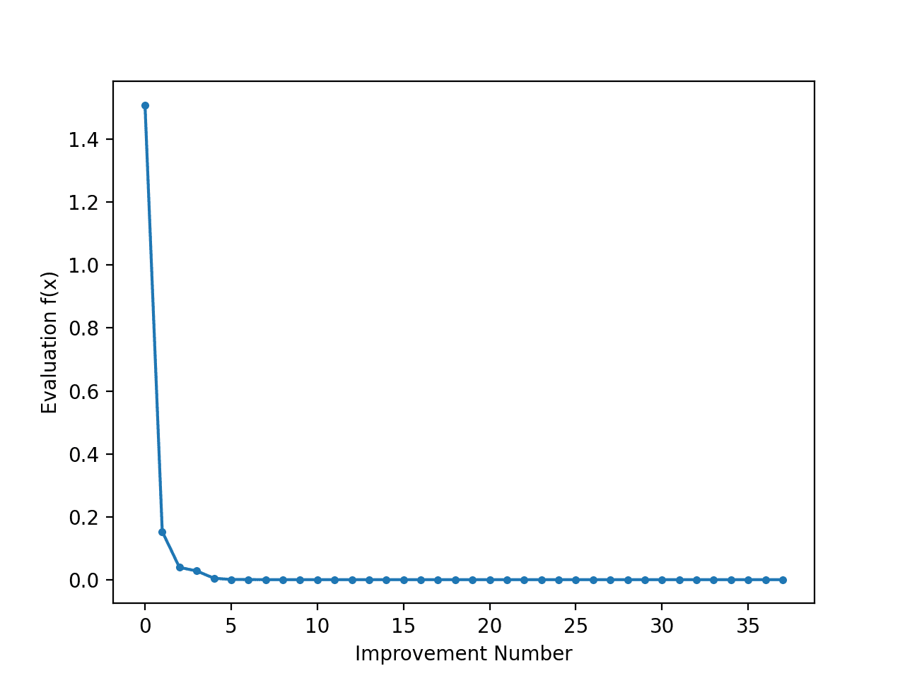
Line Plot of Objective Function Evaluation for Each Improvement During the Differential Evolution Search
Want to Get Started With Optimization Algorithms?
Take my free 7-day email crash course now (with sample code).
Click to sign-up and also get a free PDF Ebook version of the course.
Further Reading
This section provides more resources on the topic if you are looking to go deeper.
Papers
- A Simple and Efficient Heuristic for Global Optimization over Continuous Spaces, 1997.
- Recent advances in differential evolution: An updated survey, 2016.
Books
- Algorithms for Optimization, 2019.
Articles
Summary
In this tutorial, you discovered the differential evolution algorithm.
Specifically, you learned:
- Differential evolution is a heuristic approach for the global optimisation of nonlinear and non- differentiable continuous space functions.
- How to implement the differential evolution algorithm from scratch in Python.
- How to apply the differential evolution algorithm to a real-valued 2D objective function.
Get a Handle on Modern Optimization Algorithms!

Develop Your Understanding of Optimization
...with just a few lines of python code
Discover how in my new Ebook:
Optimization for Machine Learning
It provides self-study tutorials with full working code on:
Gradient Descent, Genetic Algorithms, Hill Climbing, Curve Fitting, RMSProp, Adam,
and much more...


Hi, I’m getting a list index out of range on pyplot.plot(solution[2], ‘.-‘)
Any ideas?
Sorry to hear that, perhaps some of these tips will help:
https://machinelearningmastery.com/faq/single-faq/why-does-the-code-in-the-tutorial-not-work-for-me
Hi Jason,
Thank you for the tutorial. I see so much future on these Differential Evolution and Genetic Algorithms to look for global optimization !
I did not have so much time to play with this tutorial about Differential Evolution code, but I already play with the scipy API : differential_evolution(). So I think this tutorial is just talking about buiding your own code (from scratch) algorithm. ok?
Anyway I give more attention to your previous: Genetic Algorithm (from scratch) :https://machinelearningmastery.com/simple-genetic-algorithm-from-scratch-in-python/
So, the first question I see both of them (Genetic Algorithm and Differential Evolution code) very very similar in process if not completely equal.
The only thing I see is that the mutation process is performed over a binary version on variables in genetic algorithm and here in DE not . Also I see the pattern strategy DE/x/y/z ..Am I right?
The second question is due to this process (genetic & diff evolution) are focus into get global optimum …and are so quickly, stables and efficient convergents to the global optimum…. that I guest someone must be playing with them to “replace” back-propagation or Stochastic Gradient descent to have a new option to get ML/DL model weights’s update, am I right?
thanks
How new solutions are created and the representation used are the main differences.
Yes, but generally backprop/SGD is a better solution for neural bets.
Hi,
the text says for the mutation a + F * (b – c), but the code is written as
def mutation(x, F):
return x[0] + F * x[1] – x[2]
cheers
Thanks.
Dear Dr Jason,
Another way is to go to the “complete code’. At the top of the code, there is an icon which looks like “” which opens the plain code. Copy the the code by pressing CTRL+A and then CTRL+C.
Then open a DOS window and type python to run the python interpreter under DOS.
Paste code and at the end of the last line at pyplot.show(), press enter.
I tried it and the code works.
Alternatively, run an interpreter such as “Spyder”, NOT the Idle IDE.
Paste the code = Ctrl+V.
It works.
Thank you,
Anthony of Sydney.
Dear Dr Jason,
The icon looks like that toggles between plain code and line-numbered code.
Don’t know why the disappeared when enclosed in quote marks.
So the toggle between plain code and line-numbered code by clicking on the icon.
Thank you,
Anthony of Sydney
Sorry I was referring to the icon that looked like which toggles plain coder and line-numbered code. It disappeared.
Thank you,
Anthony of Sydney
The icon is a combination of the gt (greater than) sign and lt (less than). The image of the icon is lt gt.
For an inexpllicable reason, the actual gt and lt signs don’t appear. The use of the signs look like the toggle between plain code and numbered code.
Thank you,
Anthony of Sydney
Thanks for sharing.
Dear Dr Jason,
In your tutorial, you had an objective function
What if you have a set of data and don’t know the objective function? How does one determine the objective function from raw data?
Thank you,
Anthony of Sydney
In machine learning, the objective function is often a loss function, e.g. minimizing loss of the model when making predictions on a training dataset.
Dear Dr Jason,
How do we extract the loss function to use in this differential evolution algorithm?
Thank you,
Anthony of Sydney
What do you mean by “extract the loss function”?
Generally, you define a loss function you want to minimize in machine learning, typically an error function for a model against a training dataset.
Dear Dr Jason,
I want to be able to use the loss function from any of the ML functions xgboost, keras and plug that into the differential evolution algorithm in case the cost functions from the ML algorithms in xgboost and keras have a non-differentiable function.
That is why I want to be able to extract the cost functions from the xgboost and keras and plug it in the differential evolution algorithm.
Thank you,
Anthony of Sydney
Yes, it is as I stated, the loss between the predictions and expected values in the training dataset.
You may need to write custom code to use arbitrary optimization algorithms with GBDT or neural nets.
Dear Dr Jason,
Thank you for your reply.
Three ways of asking the same question – no need to concern using differential evolution if using packages such as Keras, XGBoost, and Torch which have their own optimization techniques.
* So I can conclude that when using ML algorithms in Keras, XGBoost and Torch to name a few ML packages, there is no real need to use differential evolution?
* In other words, the differential evolution algorithms in this tutorial and at https://docs.scipy.org/doc/scipy/reference/generated/scipy.optimize.differential_evolution.html are for known functions that cannot be differentiated.
* In other words, it’s pointless using the differential evolution for known packages, Keras, XGBoostr and Torch etc.
Always appreciating your answers,
Thank you,
Anthony of Sydney
Not pointless, but you need a good reason. The conventional methods used for each algorithm are the best known methods.
Dear Dr Jason,
Thank you for your reply.
Anthony of Sydney
You’re welcome.
If I want to optimize more than one output at the same time, how can I do it?
If what you are after is solving a multi-objective optimization problem using DE, then there are several ways to do it: (paper). In essence, and quoting from the paper, “Before the evaluation of the objective function, the latter method multiplies weight to each of the objectives based on the relative importance of the objectives. Then form a new objective function by summing the weighted objectives. Thus it converts multi objectives in to single objective.“
Suppose my objective function is relative – I can tell that x is less fit than y, but I cannot score them directly with a scalar – which adjustments will be required for this to work? Or is there another evolutionary algorithm I should try?
That’s difficult but I would try to ask myself, why I would tell x is less fit than y? If you can give a logic on this, you can come up with a scalar measure.
Suppose you are learning how to play chess, and you compare players by letting them play against each other for a few games. You can say “X won against Y in 8/10 games so X is better”, but giving them a scalar value is rather meaningless – especially because this ordering is not necessarily transitive(the ordering X > Y, Y > Z, Z > X is possible). You can have the entire population play against the entire population – in this scheme the fitness is, say, 1 point for victory and -1 for a defeat. The problem is that it requires population_size^2 * k games each generation.
In real life tournaments, chess players are given ELO that represents an estimation for their likelihood to win. I experimented a little with that but since unfit genomes get eliminated, the average ELO keeps creeping up, and normalizing it rendered the whole scheme almost useless. I also suspect that the relatively small size of the simulated population also plays a part here. Perhaps that is possible, but it is so far from being trivial that I wonder if it’s worth it.
This problem is also tricky because there is no measurable objective, so It’s hard to compare different experiments, and hard to evaluate your solution (except for local convergence, which might be a “red queen” problem).
Every model has some assumption. Should this assumption violated, you can’t expect the model to work. I think it is the situation here. If X>Y, Y>Z, Z>X, then why not I can claim Y>X? This hints that you may run into a problem under the assumptions.
If I understood you correctly – you assumed X > Y, which contradicts your claim that Y > X.
Imagine a game of rock-paper-scissors.
X always plays rock
Y always plays paper
Z always player scissors
X > Z > Y > X
Which goes to show that ordering this relation through a scalar will not hold.
Note that rock-paper-scissors is an uninteresting game in which – without prior knowledge of the opponent – all strategies are equally fit, but the same situation can happen in all sort of games.
Hey Jason how can I adapt this for more than 2 X , like if my X has X1,X2…Xn?Ex: [1,2,3,4]
That would be great!? If you could help me out on that.
Hi Agrover112…Please specify the portion of the coding you wish to modify and why.
Hi, thanks a lot for the straightforward and accurate implementation of the algorithm.
I just noticed you didn’t have to calculate the “obj_target” in the inner loop for each individual (obj_target = obj(pop[j])) since it’s the same as “obj_all[j]”. Although it’s a trivial issue but it becomes quite costly when we’re evaluating a large model, like a large CNN in the case of my research.
Thanks again
Hi Hadi…You are very welcome! Thank you for the update on your progress!