Differential and Integral Calculus – Differentiate with Respect to Anything

Integral calculus was one of the greatest discoveries of Newton and Leibniz. Their work independently led to the proof, and recognition of the importance of the fundamental theorem of calculus, which linked integrals to derivatives. With the discovery of integrals, areas and volumes could thereafter be studied. 

Integral calculus is the second half of the calculus journey that we will be exploring.

In this tutorial, you will discover the relationship between differential and integral calculus. 

After completing this tutorial, you will know:

• The concepts of differential and integral calculus are linked together by the fundamental theorem of calculus. 
• By applying the fundamental theorem of calculus, we can compute the integral to find the area under a curve. 
• In machine learning, the application of integral calculus can provide us with a metric to assess the performance of a classifier. 

Let’s get started. 

Differential and Integral Calculus – Differentiate with Respect to Anything
Photo by Maxime Lebrun, some rights reserved.

Tutorial Overview

This tutorial is divided into three parts; they are:

• Differential and Integral Calculus – What is the Link?
• The Fundamental Theorem of Calculus
  • The Sweeping Area Analogy
  • The Fundamental Theorem of Calculus – Part 1
  • The Fundamental Theorem of Calculus – Part 2
• Integration Example
• Application of Integration in Machine Learning

Differential and Integral Calculus – What is the Link?

In our journey through calculus so far, we have learned that differential calculus is concerned with the measurement of the rate of change. We have also discovered differentiation, and applied it to different functions from first principles. We have even understood how to apply rules to arrive to the derivative faster. 

But we are only half way through the journey. 

From A twenty-first-century vantage point, calculus is often seen as the mathematics of change. It quantifies change using two big concepts: derivatives and integrals. Derivatives model rates of change … Integrals model the accumulation of change …

– Page 141, Infinite Powers, 2020.

Recall having said that calculus comprises two phases: cutting and rebuilding.  

The cutting phase breaks down a curved shape into infinitesimally small and straight pieces that can be studied separately, such as by applying derivatives to model their rate of change, or slope. 

This half of the calculus journey is called differential calculus, and we have already looked into it in some detail. 

The rebuilding phase gathers the infinitesimally small and straight pieces, and sums them back together in an attempt to study the original whole. In this manner, we can determine the area or volume of regular and irregular shapes after having cut them into infinitely thin slices. This second half of the calculus journey is what we shall be exploring next. It is called integral calculus.

The important theorem that links the two concepts together is called the fundamental theorem of calculus. 

The Fundamental Theorem of Calculus

In order to work our way towards understanding the fundamental theorem of calculus, let’s revisit the car’s position and velocity example: 

Line Plot of the Car’s Position Against Time

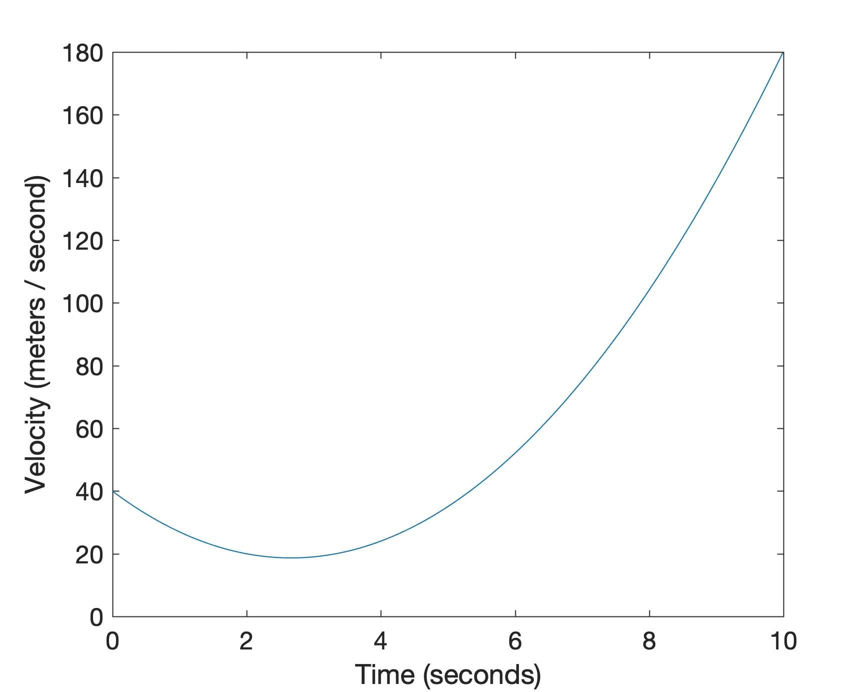
Line Plot of the Car’s Velocity Against Time

In computing the derivative we had solved the forward problem, where we found the velocity from the slope of the position graph at any time, t. But what if we would like to solve the backward problem, where we are given the velocity graph, v(t), and wish to find the distance travelled? The solution to this problem is to calculate the area under the curve (the shaded region) up to time, t:

The Shaded Region is the Area Under the Curve

We do not have a specific formula to define the area of the shaded region directly. But we can apply the mathematics of calculus to cut the shaded region under the curve into many infinitely thin rectangles, for which we have a formula:

Cutting the Shaded Region Into Many Rectangles of Width, Δt

If we consider the i^th rectangle, chosen arbitrarily to span the time interval Δt, we can define its area as its length times its width:

area_of_rectangle = v(t_i) Δt_i

We can have as many rectangles as necessary in order to span the interval of interest, which in this case is the shaded region under the curve. For simplicity, let’s denote this closed interval by [a, b]. Finding the area of this shaded region (and, hence, the distance travelled), then reduces to finding the sum of the n number of rectangles:

total_area = v(t₀) Δt₀ + v(t₁) Δt₁ + … + v(t_n) Δt_n

We can express this sum even more compactly by applying the Riemann sum with sigma notation:

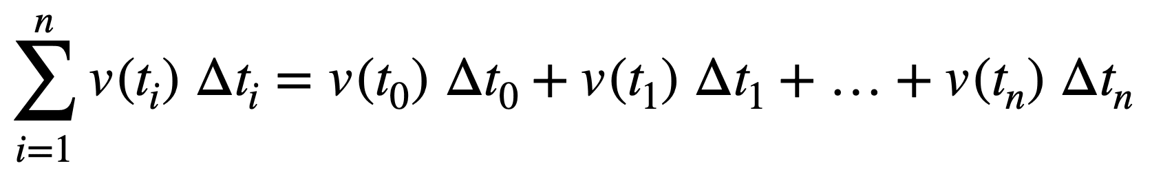
If we cut (or divide) the region under the curve by a finite number of rectangles, then we find that the Riemann sum gives us an approximation of the area, since the rectangles will not fit the area under the curve exactly. If we had to position the rectangles so that their upper left or upper right corners touch the curve, the Riemann sum gives us either an underestimate or an overestimate of the true area, respectively. If the midpoint of each rectangle had to touch the curve, then the part of the rectangle protruding above the curve roughly compensates for the gap between the curve and neighbouring rectangles:

Approximating the Area Under the Curve with Left Sums

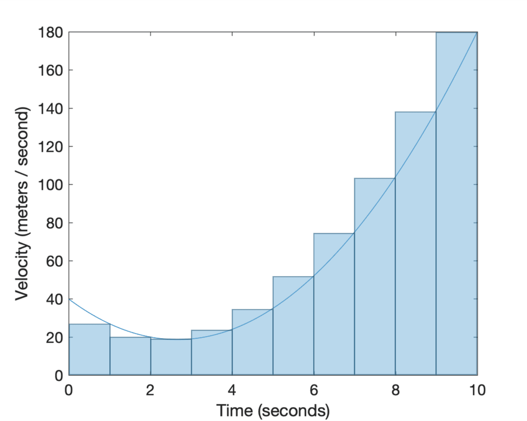
Approximating the Area Under the Curve with Right Sums

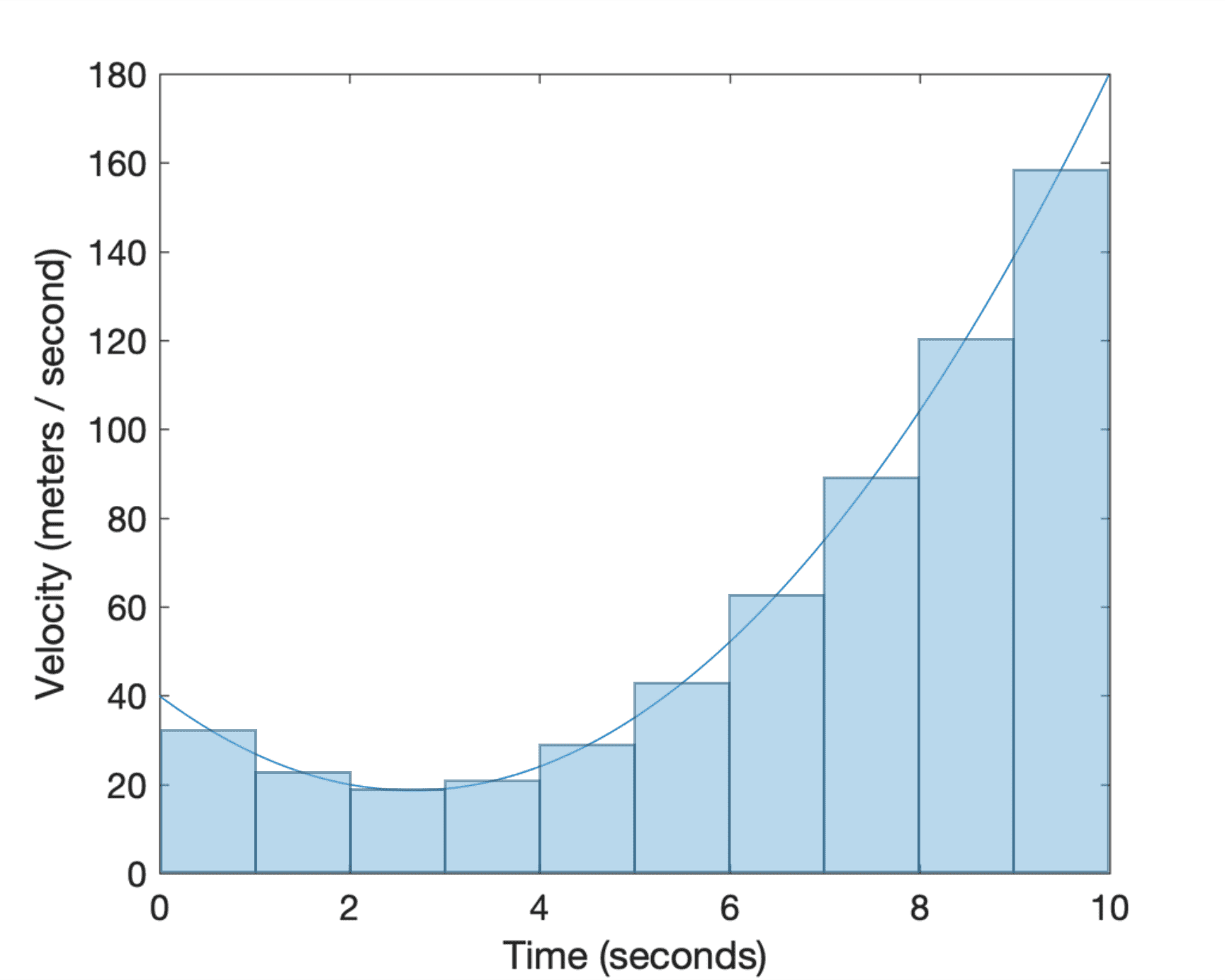
Approximating the Area Under the Curve with Midpoint Sums

The solution to finding the exact area under the curve, is to reduce the rectangles’ width so much that they become infinitely thin (recall the Infinity Principle in calculus). In this manner, the rectangles would be covering the entire region, and in summing their areas we would be finding the definite integral. 

The definite integral (“simple” definition): The exact area under a curve between t = a and t = b is given by the definite integral, which is defined as the limit of a Riemann sum …

– Page 227, Calculus for Dummies, 2016.

The definite integral can, then, be defined by the Riemann sum as the number of rectangles, n, approaches infinity. Let’s also denote the area under the curve by A(t). Then:

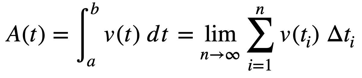
Note that the notation now changes into the integral symbol, ∫, replacing sigma, Σ. The reason behind this change is, merely, to indicate that we are summing over a huge number of thinly sliced rectangles. The expression on the left hand side reads as, the integral of v(t) from a to b, and the process of finding the integral is called integration.  

The Sweeping Area Analogy

Perhaps a simpler analogy to help us relate integration to differentiation, is to imagine holding one of the thinly cut slices and dragging it rightwards under the curve in infinitesimally small steps. As it moves rightwards, the thinly cut slice will sweep a larger area under the curve, while its height will change according to the shape of the curve. The question that we would like to answer is, at which rate does the area accumulate as the thin slice sweeps rightwards?

Let dt denote each infinitesimal step traversed by the sweeping slice, and v(t) its height at any time, t. Then the infinitesimal area, dA(t), of this thin slice can be found by multiplying its height, v(t), to its infinitesimal width, dt:

dA(t) = v(t) dt

Dividing the equation by dt gives us the derivative of A(t), and tells us that the rate at which the area accumulates is equal to the height of the curve, v(t), at time, t:

dA(t) / dt = v(t)

We can finally define the fundamental theorem of calculus. 

The Fundamental Theorem of Calculus – Part 1

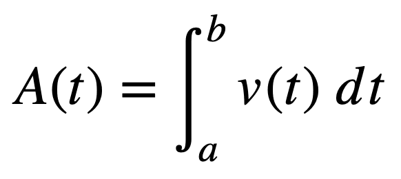
We found that an area, A(t), swept under a function, v(t), can be defined by:

We have also found that the rate at which the area is being swept is equal to the original function, v(t):

dA(t) / dt = v(t)

This brings us to the first part of the fundamental theorem of calculus, which tells us that if v(t) is  continuous on an interval, [a, b], and if it is also the derivative of A(t), then A(t) is the antiderivative of v(t):

 A’(t) = v(t)

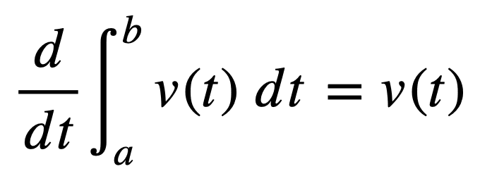
Or in simpler terms, integration is the reverse operation of differentiation. Hence, if we first had to integrate v(t) and then differentiate the result, we would get back the original function, v(t):

The Fundamental Theorem of Calculus – Part 2

The second part of the theorem gives us a shortcut for computing the integral, without having to take the longer route of computing the limit of a Riemann sum. 

It states that if the function, v(t), is continuous on an interval, [a, b], then:

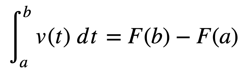
Here, F(t) is any antiderivative of v(t), and the integral is defined as the subtraction of the antiderivative evaluated at a and b. 

Hence, the second part of the theorem computes the integral by subtracting the area under the curve between some starting point, C, and the lower limit, a, from the area between the same starting point, C, and the upper limit, b. This, effectively, calculates the area of interest between a and b. 

Since the constant, C, defines the point on the x-axis at which the sweep starts, the simplest antiderivative to consider is the one with C = 0. Nonetheless, any antiderivative with any value of C can be used, which simply sets the starting point to a different position on the x-axis. 

Integration Example

Consider the function, v(t) = x³. By applying the power rule, we can easily find its derivative, v’(t) = 3x². The antiderivative of 3x² is again x³ – we perform the reverse operation to obtain the original function.

Now suppose that we have a different function, g(t) = x³ + 2. Its derivative is also 3x², and so is the derivative of yet another function, h(t) = x³ – 5. Both of these functions (and other similar ones) have x³ as their antiderivative. Hence, we specify the family of all antiderivatives of 3x² by the indefinite integral:

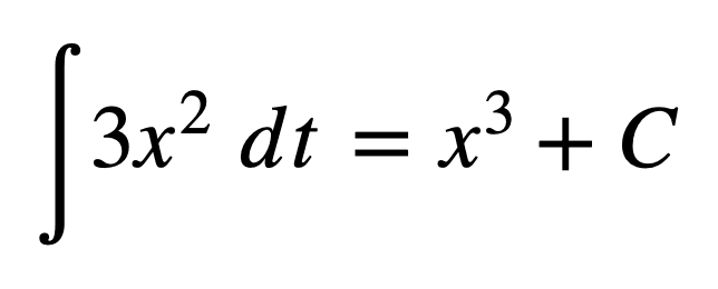
The indefinite integral does not define the limits between which the area under the curve is being calculated. The constant, C, is included to compensate for the lack of information about the limits, or the starting point of the sweep.

If we do have knowledge of the limits, then we can simply apply the second fundamental theorem of calculus to compute the definite integral:

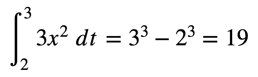
 We can simply set C to zero, because it will not change the result in this case. 

Application of Integration in Machine Learning

We have considered the car’s velocity curve, v(t), as a familiar example to understand the relationship between integration and differentiation. 

But you can use this adding-up-areas-of-rectangles scheme to add up tiny bits of anything — distance, volume, or energy, for example. In other words, the area under the curve doesn’t have to stand for an actual area. 

 – Page 214, Calculus for Dummies, 2016.

One of the important steps of successfully applying machine learning techniques includes the choice of appropriate performance metrics. In deep learning, for instance, it is common practice to measure precision and recall.

Precision is the fraction of detections reported by the model that were correct, while recall is the fraction of true events that were detected. 

– Page 423, Deep Learning, 2017.

It is also common practice to, then, plot the precision and recall on a Precision-Recall (PR) curve, placing the recall on the x-axis and the precision on the y-axis. It would be desirable that a classifier is characterised by both high recall and high precision, meaning that the classifier can detect many of the true events correctly. Such a good classification performance would be characterised by a higher area under the PR curve. 

You can probably already tell where this is going. 

The area under the PR curve can, indeed, be calculated by applying integral calculus, permitting us to characterise the performance of the classifier. 

Further Reading

This section provides more resources on the topic if you are looking to go deeper.

Books

• Single and Multivariable Calculus, 2020.
• Calculus for Dummies, 2016.
• Infinite Powers, 2020.
• The Hitchhiker’s Guide to Calculus, 2019.
• Deep Learning, 2017.

Summary

In this tutorial, you discovered the relationship between differential and integral calculus.

Specifically, you learned:

• The concepts of differential and integral calculus are linked together by the fundamental theorem of calculus. 
• By applying the fundamental theorem of calculus, we can compute the integral to find the area under a curve. 
• In machine learning, the application of integral calculus can provide us with a metric to assess the performance of a classifier.  

Do you have any questions?
Ask your questions in the comments below and I will do my best to answer.

Get a Handle on Calculus for Machine Learning!

Feel Smarter with Calculus Concepts

...by getting a better sense on the calculus symbols and terms

Discover how in my new Ebook:
Calculus for Machine Learning

It provides self-study tutorials with full working code on:
differntiation, gradient, Lagrangian mutiplier approach, Jacobian matrix, and much more...

Bring Just Enough Calculus Knowledge to
Your Machine Learning Projects

See What's Inside