A Gentle Introduction to the Jacobian

In the literature, the term Jacobian is often interchangeably used to refer to both the Jacobian matrix or its determinant. 

Both the matrix and the determinant have useful and important applications: in machine learning, the Jacobian matrix aggregates the partial derivatives that are necessary for backpropagation; the determinant is useful in the process of changing between variables.

In this tutorial, you will review a gentle introduction to the Jacobian. 

After completing this tutorial, you will know:

• The Jacobian matrix collects all first-order partial derivatives of a multivariate function that can be used for backpropagation.
• The Jacobian determinant is useful in changing between variables, where it acts as a scaling factor between one coordinate space and another. 

Let’s get started. 

A Gentle Introduction to the Jacobian
Photo by Simon Berger, some rights reserved.

Tutorial Overview

This tutorial is divided into three parts; they are:

• Partial Derivatives in Machine Learning
• The Jacobian Matrix
• Other Uses of the Jacobian

Partial Derivatives in Machine Learning

We have thus far mentioned gradients and partial derivatives as being important for an optimization algorithm to update, say, the model weights of a neural network to reach an optimal set of weights. The use of partial derivatives permits each weight to be updated independently of the others, by calculating the gradient of the error curve with respect to each weight in turn.

Many of the functions that we usually work with in machine learning are multivariate, vector-valued functions, which means that they map multiple real inputs, n,  to multiple real outputs, m:

For example, consider a neural network that classifies grayscale images into several classes. The function being implemented by such a classifier would map the n pixel values of each single-channel input image, to m output probabilities of belonging to each of the different classes. 

In training a neural network, the backpropagation algorithm is responsible for sharing back the error calculated at the output layer, among the neurons comprising the different hidden layers of the neural network, until it reaches the input. 

The fundamental principle of the backpropagation algorithm in adjusting the weights in a network is that each weight in a network should be updated in proportion to the sensitivity of the overall error of the network to changes in that weight. 

– Page 222, Deep Learning, 2019.

This sensitivity of the overall error of the network to changes in any one particular weight is measured in terms of the rate of change, which, in turn, is calculated by taking the partial derivative of the error with respect to the same weight. 

For simplicity, suppose that one of the hidden layers of some particular network consists of just a single neuron, k. We can represent this in terms of a simple computational graph:

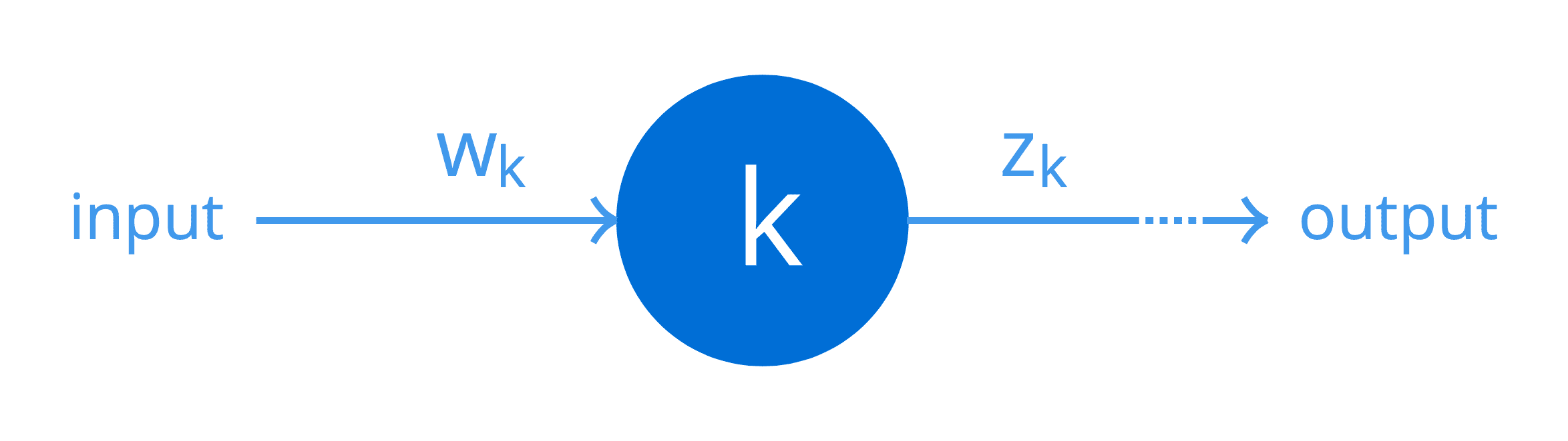
A Neuron with a Single Input and a Single Output

Again, for simplicity, let’s suppose that a weight, w_k, is applied to an input of this neuron to produce an output, z_k, according to the function that this neuron implements (including the nonlinearity). Then, the weight of this neuron can be connected to the error at the output of the network as follows (the following formula is formally known as the chain rule of calculus, but more on this later in a separate tutorial):

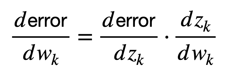
Here, the derivative, dz_k / dw_k, first connects the weight, w_k, to the output, z_k, while the derivative, derror / dz_k, subsequently connects the output, z_k, to the network error. 

It is more often the case that we’d have many connected neurons populating the network, each attributed a different weight. Since we are more interested in such a scenario, then we can generalise beyond the scalar case to consider multiple inputs and multiple outputs:

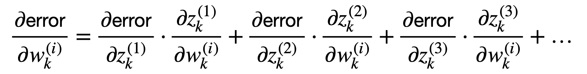
This sum of terms can be represented more compactly as follows:

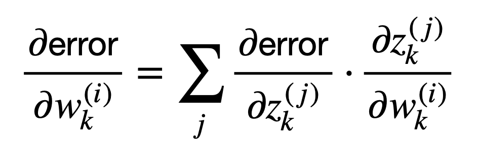
Or, equivalently, in vector notation using the del operator, ∇, to represent the gradient of the error with respect to either the weights, w_k, or the outputs, z_k:

The back-propagation algorithm consists of performing such a Jacobian-gradient product for each operation in the graph.

– Page 207, Deep Learning, 2017.

This means that the backpropagation algorithm can relate the sensitivity of the network error to changes in the weights, through a multiplication by the Jacobian matrix, (∂z_k / ∂w_k)^T.

Hence, what does this Jacobian matrix contain?

The Jacobian Matrix

The Jacobian matrix collects all first-order partial derivatives of a multivariate function.

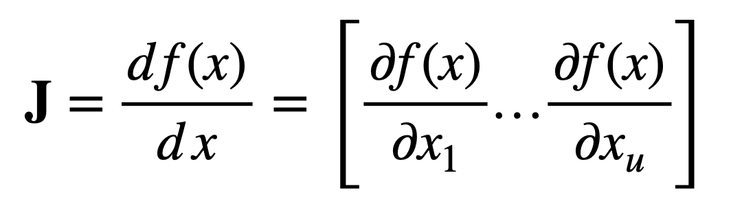
Specifically, consider first a function that maps u real inputs, to a single real output:

Then, for an input vector, x, of length, u, the Jacobian vector of size, 1 × u, can be defined as follows:

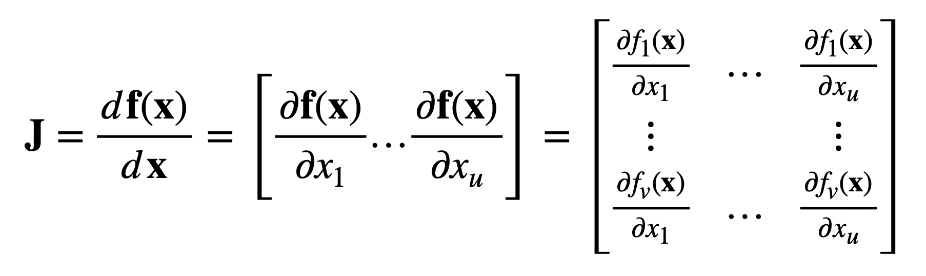
Now, consider another function that maps u real inputs, to v real outputs:

Then, for the same input vector, x, of length, u, the Jacobian is now a v × u matrix, J ∈ ℝ^v×u, that is defined as follows:

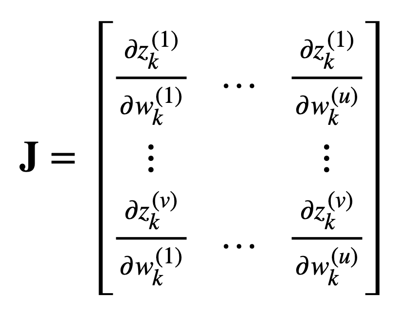
Reframing the Jacobian matrix into the machine learning problem considered earlier, while retaining the same number of u real inputs and v real outputs, we find that this matrix would contain the following partial derivatives:

Other Uses of the Jacobian

An important technique when working with integrals involves the change of variables (also referred to as, integration by substitution or u-substitution), where an integral is simplified into another integral that is easier to compute. 

In the single variable case, substituting some variable, x, with another variable, u, can transform the original function into a simpler one for which it is easier to find an antiderivative. In the two variable case, an additional reason might be that we would also wish to transform the region of terms over which we are integrating, into a different shape. 

In the single variable case, there’s typically just one reason to want to change the variable: to make the function “nicer” so that we can find an antiderivative. In the two variable case, there is a second potential reason: the two-dimensional region over which we need to integrate is somehow unpleasant, and we want the region in terms of u and v to be nicer—to be a rectangle, for example. 

– Page 412, Single and Multivariable Calculus, 2020.

When performing a substitution between two (or possibly more) variables, the process starts with a definition of the variables between which the substitution is to occur. For example, x = f(u, v) and y = g(u, v). This is then followed by a conversion of the integral limits depending on how the functions, f and g, will transform the u–v plane into the x–y plane. Finally, the absolute value of the Jacobian determinant is computed and included, to act as a scaling factor between one coordinate space and another. 

Further Reading

This section provides more resources on the topic if you are looking to go deeper.

Books

• Deep Learning, 2017.
• Mathematics for Machine Learning, 2020.
• Single and Multivariable Calculus, 2020.
• Deep Learning, 2019.

Articles

• Jacobian matrix and determinant, Wikipedia.
• Integration by substitution, Wikipedia.

Summary

In this tutorial, you discovered a gentle introduction to the Jacobian.

Specifically, you learned:

• The Jacobian matrix collects all first-order partial derivatives of a multivariate function that can be used for backpropagation.
• The Jacobian determinant is useful in changing between variables, where it acts as a scaling factor between one coordinate space and another.

Do you have any questions?
Ask your questions in the comments below and I will do my best to answer.

Get a Handle on Calculus for Machine Learning!

Feel Smarter with Calculus Concepts

...by getting a better sense on the calculus symbols and terms

Discover how in my new Ebook:
Calculus for Machine Learning

It provides self-study tutorials with full working code on:
differntiation, gradient, Lagrangian mutiplier approach, Jacobian matrix, and much more...

Bring Just Enough Calculus Knowledge to
Your Machine Learning Projects

See What's Inside