Calculus for Machine Learning (7-day mini-course)

Calculus for Machine Learning Crash Course.
Get familiar with the calculus techniques in machine learning in 7 days.

Calculus is an important mathematics technique behind many machine learning algorithms. You don’t always need to know it to use the algorithms. When you go deeper, you will see it is ubiquitous in every discussion on the theory behind a machine learning model.

As a practitioner, we are most likely not going to encounter very hard calculus problems. If we need to do one, there are tools such as computer algebra systems to help, or at least, verify our solution. However, what is more important is understanding the idea behind calculus and relating the calculus terms to its use in our machine learning algorithms.

In this crash course, you will discover some common calculus ideas used in machine learning. You will learn with exercises in Python in seven days.

This is a big and important post. You might want to bookmark it.

Let’s get started.

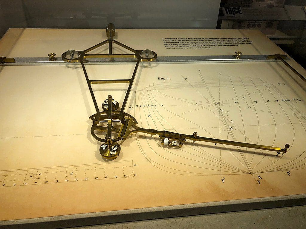
Calculus for Machine Learning (7-Day Mini-Course)
Photo by ArnoldReinhold, some rights reserved.

Who Is This Crash-Course For?

Before we get started, let’s make sure you are in the right place.

This course is for developers who may know some applied machine learning. Maybe you know how to work through a predictive modeling problem end to end, or at least most of the main steps, with popular tools.

The lessons in this course do assume a few things about you, such as:

• You know your way around basic Python for programming.
• You may know some basic linear algebra.
• You may know some basic machine learning models.

You do NOT need to be:

• A math wiz!
• A machine learning expert!

This crash course will take you from a developer who knows a little machine learning to a developer who can effectively talk about the calculus concepts in machine learning algorithms.

Note: This crash course assumes you have a working Python 3.7 environment with some libraries such as SciPy and SymPy installed. If you need help with your environment, you can follow the step-by-step tutorial here:

• How to Set Up Your Python Environment for Machine Learning With Anaconda

Crash-Course Overview

This crash course is broken down into seven lessons.

You could complete one lesson per day (recommended) or complete all of the lessons in one day (hardcore). It really depends on the time you have available and your level of enthusiasm.

Below is a list of the seven lessons that will get you started and productive with data preparation in Python:

• Lesson 01: Differential calculus
• Lesson 02: Integration
• Lesson 03: Gradient of a vector function
• Lesson 04: Jacobian
• Lesson 05: Backpropagation
• Lesson 06: Optimization
• Lesson 07: Support vector machine

Each lesson could take you 5 minutes or up to 1 hour. Take your time and complete the lessons at your own pace. Ask questions, and even post results in the comments below.

The lessons might expect you to go off and find out how to do things. I will give you hints, but part of the point of each lesson is to force you to learn where to go to look for help with and about the algorithms and the best-of-breed tools in Python. (Hint: I have all of the answers on this blog; use the search box.)

Post your results in the comments; I’ll cheer you on!

Hang in there; don’t give up.

Lesson 01: Differential Calculus

In this lesson, you will discover what is differential calculus or differentiation.

Differentiation is the operation of transforming one mathematical function to another, called the derivative. The derivative tells the slope, or the rate of change, of the original function.

For example, if we have a function $f(x)=x^2$, its derivative is a function that tells us the rate of change of this function at $x$. The rate of change is defined as: $$f'(x) = \frac{f(x+\delta x)-f(x)}{\delta x}$$ for a small quantity $\delta x$.

Usually we will define the above in the form of a limit, i.e.,

$$f'(x) = \lim_{\delta x\to 0} \frac{f(x+\delta x)-f(x)}{\delta x}$$

to mean $\delta x$ should be as close to zero as possible.

There are several rules of differentiation to help us find the derivative easier. One rule that fits the above example is $\frac{d}{dx} x^n = nx^{n-1}$. Hence for $f(x)=x^2$, we have the derivative $f'(x)=2x$.

We can confirm this is the case by plotting the function $f'(x)$ computed according to the rate of change together with that computed according to the rule of differentiation. The following uses NumPy and matplotlib in Python:

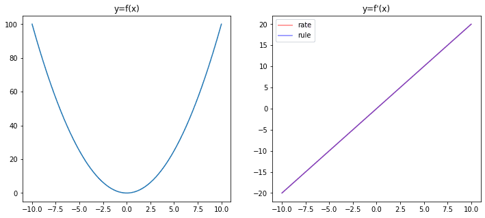
In the plot above, we can see the derivative function found using the rate of change and then using the rule of differentiation coincide perfectly.

Your Task

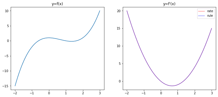
We can similarly do a differentiation of other functions. For example, $f(x)=x^3 – 2x^2 + 1$. Find the derivative of this function using the rules of differentiation and compare your result with the result found using the rate of limits. Verify your result with the plot above. If you’re doing it correctly, you should see the following graph:

In the next lesson, you will discover that integration is the reverse of differentiation.

Lesson 02: Integration

In this lesson, you will discover integration is the reverse of differentiation.

If we consider a function $f(x)=2x$ and at intervals of $\delta x$ each step (e.g., $\delta x = 0.1$), we can compute, say, from $x=-10$ to $x=10$ as:

$$
f(-10), f(-9.9), f(-9.8), \cdots, f(9.8), f(9.9), f(10)
$$

Obviously, if we have a smaller step $\delta x$, there are more terms in the above.

If we multiply each of the above with the step size and then add them up, i.e.,

$$
f(-10)\times 0.1 + f(-9.9)\times 0.1 + \cdots + f(9.8)\times 0.1 + f(9.9)\times 0.1
$$

this sum is called the integral of $f(x)$. In essence, this sum is the area under the curve of $f(x)$, from $x=-10$ to $x=10$. A theorem in calculus says if we put the area under the curve as a function, its derivative is $f(x)$. Hence we can see the integration as a reverse operation of differentiation.

As we saw in Lesson 01, the differentiation of $f(x)=x^2$ is $f'(x)=2x$. This means for $f(x)=2x$, we can write $\int f(x) dx = x^2$ or we can say the antiderivative of $f(x)=x$ is $x^2$. We can confirm this in Python by calculating the area directly:

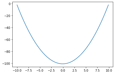
This plot has the same shape as $f(x)$ in Lesson 01. Indeed, all functions differ by a constant (e.g., $f(x)$ and $f(x)+5$) that have the same derivative. Hence the plot of the antiderivative computed will be the original shifted vertically.

Your Task

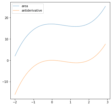
Consider $f(x)=3x^2-4x$, find the antiderivative of this function and plot it. Also, try to replace the Python code above with this function. If you plot both together, you should see the following:

Post your answer in the comments below. I would love to see what you come up with.

Lesson 03: Gradient of a vector function

In this lesson, you will learn the concept of gradient of a multivariate function.

If we have a function of not one variable but two or more, the differentiation is extended naturally to be the differentiation of the function with respect to each variable. For example, if we have the function $f(x,y) = x^2 + y^3$, we can write the differentiation in each variable as:

$$
\begin{aligned}
\frac{\partial f}{\partial x} &= 2x \\
\frac{\partial f}{\partial y} &= 3y^2
\end{aligned}
$$

Here we introduced the notation of a partial derivative, meaning to differentiate a function on one variable while assuming the other variables are constants. Hence in the above, when we compute $\frac{\partial f}{\partial x}$, we ignored the $y^3$ part in the function $f(x,y)$.

A function with two variables can be visualized as a surface on a plane. The above function $f(x,y)$ can be visualized using matplotlib:

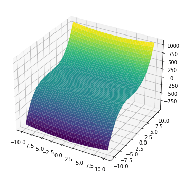
The gradient of this function is denoted as:

$$\nabla f(x,y) = \Big(\frac{\partial f}{\partial x},\; \frac{\partial f}{\partial y}\Big) = (2x,\;3y^2)$$

Therefore, at each coordinate $(x,y)$, the gradient $\nabla f(x,y)$ is a vector. This vector tells us two things:

• The direction of the vector points to where the function $f(x,y)$ is increasing the fastest
• The size of the vector is the rate of change of the function $f(x,y)$ in this direction

One way to visualize the gradient is to consider it as a vector field:

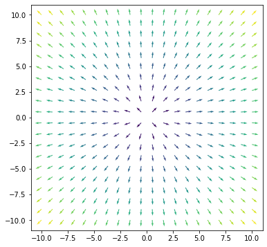
The viridis color map in matplotlib will show a larger value in yellow and a lower value in purple. Hence we see the gradient is “steeper” at the edges than in the center in the above plot.

If we consider the coordinate (2,3), we can check which direction $f(x,y)$ will increase the fastest using the following:

Its output is:

The gradient vector according to the formula is (4,27), which the numerical result above is close enough.

Your Task

Consider the function $f(x,y)=x^2+y^2$, what is the gradient vector at (1,1)? If you get the answer from partial differentiation, can you modify the above Python code to confirm it by checking the rate of change at different directions?

Post your answer in the comments below. I would love to see what you come up with.

In the next lesson, you will discover the differentiation of a function that takes vector input and produces vector output.

Lesson 04: Jacobian

In this lesson, you will learn about Jacobian matrix.

The function $f(x,y)=(p(x,y), q(x,y))=(2xy, x^2y)$ is one with two input and two outputs. Sometimes we call this function taking vector arguments and returning a vector value. The differentiation of this function is a matrix called the Jacobian. The Jacobian of the above function is:

$$
\mathbf{J} =
\begin{bmatrix}
\frac{\partial p}{\partial x} & \frac{\partial p}{\partial y} \\
\frac{\partial q}{\partial x} & \frac{\partial q}{\partial y}
\end{bmatrix}
=
\begin{bmatrix}
2y & 2x \\
2xy & x^2
\end{bmatrix}
$$

In the Jacobian matrix, each row has the partial differentiation of each element of the output vector, and each column has the partial differentiation with respect to each element of the input vector.

We will see the use of Jacobian later. Since finding a Jacobian matrix involves a lot of partial differentiations, it would be great if we could let a computer check our math. In Python, we can verify the above result using SymPy:

Its output is:

We asked SymPy to define the symbols x and y and then defined the vector function f. Afterward, the Jacobian can be found by calling the jacobian() function.

Your Task

Consider the function
$$
f(x,y) = \begin{bmatrix}
\frac{1}{1+e^{-(px+qy)}} & \frac{1}{1+e^{-(rx+sy)}} & \frac{1}{1+e^{-(tx+uy)}}
\end{bmatrix}
$$

where $p,q,r,s,t,u$ are constants. What is the Jacobian matrix of $f(x,y)$? Can you verify it with SymPy?

In the next lesson, you will discover the application of the Jacobian matrix in a neural network’s backpropagation algorithm.

Lesson 05: Backpropagation

In this lesson, you will see how the backpropagation algorithm uses the Jacobian matrix.

If we consider a neural network with one hidden layer, we can represent it as a function:

$$
y = g\Big(\sum_{k=1}^M u_k f_k\big(\sum_{i=1}^N w_{ik}x_i\big)\Big)
$$

The input to the neural network is a vector $\mathbf{x}=(x_1, x_2, \cdots, x_N)$ and each $x_i$ will be multiplied with weight $w_{ik}$ and fed into the hidden layer. The output of neuron $k$ in the hidden layer will be multiplied with weight $u_k$ and fed into the output layer. The activation function of the hidden layer and output layer are $f$ and $g$, respectively.

If we consider

$$z_k = f_k\big(\sum_{i=1}^N w_{ik}x_i\big)$$

then

$$
\frac{\partial y}{\partial x_i} = \sum_{k=1}^M \frac{\partial y}{\partial z_k}\frac{\partial z_k}{\partial x_i}
$$

If we consider the entire layer at once, we have $\mathbf{z}=(z_1, z_2, \cdots, z_M)$ and then

$$
\frac{\partial y}{\partial \mathbf{x}} = \mathbf{W}^\top\frac{\partial y}{\partial \mathbf{z}}
$$

where $\mathbf{W}$ is the $M\times N$ Jacobian matrix, where the element on row $k$ and column $i$ is $\frac{\partial z_k}{\partial x_i}$.

This is how the backpropagation algorithm works in training a neural network! For a network with multiple hidden layers, we need to compute the Jacobian matrix for each layer.

Your Task

The code below implements a neural network model that you can try yourself. It has two hidden layers and a classification network to separate points in 2-dimension into two classes. Try to look at the function backward() and identify which is the Jacobian matrix.

If you play with this code, the class mlp should not be modified, but you can change the parameters on how a model is created.

In the next lesson, you will discover the use of differentiation to find the optimal value of a function.

Lesson 06: Optimization

In this lesson, you will learn an important use of differentiation.

Because the differentiation of a function is the rate of change, we can make use of differentiation to find the optimal point of a function.

If a function attained its maximum, we would expect it to move from a lower point to the maximum, and if we move further, it falls to another lower point. Hence at the point of maximum, the rate of change of a function is zero. And vice versa for the minimum.

As an example, consider $f(x)=x^3-2x^2+1$. The derivative is $f'(x) = 3x^2-4x$ and $f'(x)=0$ at $x=0$ and $x=4/3$. Hence these positions of $x$ are where $f(x)$ is at its maximum or minimum. We can visually confirm it by plotting $f(x)$ (see the plot in Lesson 01).

Your task

Consider the function $f(x)=\log x$ and find its derivative. What will be the value of $x$ when $f'(x)=0$? What does it tell you about the maximum or minimum of the log function? Try to plot the function of $\log x$ to visually confirm your answer.

In the next lesson, you will discover the application of this technique in finding the support vector.

Lesson 07: Support vector machine

In this lesson, you will learn how we can convert support vector machine into an optimization problem.

In a two-dimensional plane, any straight line can be represented by the equation:

$$ax+by+c=0$$

in the $xy$-coordinate system. A result from the study of coordinate geometry says that for any point $(x_0,y_0)$, its distance to the line $ax+by+c=0$ is:

$$
\frac{\vert ax_0+by_0+c \vert}{\sqrt{a^2+b^2}}
$$

Consider the points (0,0), (1,2), and (2,1) in the $xy$-plane, in which the first point and the latter two points are in different classes. What is the line that best separates these two classes? This is the basis of a support vector machine classifier. The support vector is the line of maximum separation in this case.

To find such a line, we are looking for:

$$
\begin{aligned}
\text{minimize} && a^2 + b^2 \\
\text{subject to} && -1(0a+0b+c) &\ge 1 \\
&& +1(1a+2b+c) &\ge 1 \\
&& +1(2a+1b+c) &\ge 1
\end{aligned}
$$

The objective $a^2+b^2$ is to be minimized so that the distances from each data point to the line are maximized. The condition $-1(0a+0b+c)\ge 1$ means the point (0,0) is of class $-1$; similarly for the other two points, they are of class $+1$. The straight line should put these two classes in different sides of the plane.

This is a constrained optimization problem, and the way to solve it is to use the Lagrange multiplier approach. The first step in using the Lagrange multiplier approach is to find the partial differentials of the following Lagrange function:

$$
L = a^2+b^2 + \lambda_1(-c-1) + \lambda_2 (a+2b+c-1) + \lambda_3 (2a+b+c-1)
$$

and set the partial differentials to zero, then solve for $a$, $b$, and $c$. It would be too lengthy to demonstrate here, but we can use SciPy to find the solution to the above numerically:

It will print:

The above means the line to separate these three points is $0.67x + 0.67y – 1 = 0$. Note that if you provided $N$ data points, there would be $N$ constraints to be defined.

Your Task

Let’s consider the points (-1,-1) and (-3,-1) to be the first class together with (0,0) and point (3,3) to be the second class together with points (1,2) and (2,1). In this problem of six points, can you modify the above program and find the line that separates the two classes? Don’t be surprised to see the solution remain the same as above. There is a reason for it. Can you tell?

Post your answer in the comments below. I would love to see what you come up with.

This was the final lesson.

The End!
(Look How Far You Have Come)

You made it. Well done!

Take a moment and look back at how far you have come.

You discovered:

• What is differentiation, and what it means to a function
• What is integration
• How to extend differentiation to a function of vector argument
• How to do differentiation on a vector-valued function
• The role of Jacobian in the backpropagation algorithm in neural networks
• How to use differentiation to find the optimum points of a function
• Support vector machine is a constrained optimization problem, which would need differentiation to solve

Summary

How did you do with the mini-course?
Did you enjoy this crash course?

Do you have any questions? Were there any sticking points?
Let me know. Leave a comment below.

Get a Handle on Calculus for Machine Learning!

Feel Smarter with Calculus Concepts

...by getting a better sense on the calculus symbols and terms

Discover how in my new Ebook:
Calculus for Machine Learning

It provides self-study tutorials with full working code on:
differntiation, gradient, Lagrangian mutiplier approach, Jacobian matrix, and much more...

Bring Just Enough Calculus Knowledge to
Your Machine Learning Projects

See What's Inside