We have previously seen that calculus is one of the core mathematical concepts in machine learning that permits us to understand the internal workings of different machine learning algorithms.
Calculus, in turn, builds on several fundamental concepts that derive from algebra and geometry. The importance of having these fundamentals at hand will become even more important as we work our way through more advanced topics of calculus, such as the evaluation of limits and the computation of derivatives, to name a few.
In this tutorial, you will discover several pre-requisites that will help you work with calculus.
After completing this tutorial, you will know:
- Linear and non-linear functions are central to calculus and machine learning, and many calculus problems involve their use.
- Fundamental concepts from algebra and trigonometry provide the foundations for calculus, and will become especially important as we tackle more advanced calculus topics.
Let’s get started.

What you need to know before you get started: A brief tour of Calculus Pre-Requisites
Photo by Dino Reichmuth, some rights reserved.
Tutorial Overview
This tutorial is divided into three parts; they are:
- The Concept of a Function
- Fundamentals of Pre-Algebra and Algebra
- Fundamentals of Trigonometry
The Concept of a Function
A function is a rule that defines the relationship between a dependent variable and an independent variable.
Examples are all around us: The average daily temperature for your city depends on, and is a function of, the time of year; the distance an object has fallen is a function of how much time has elapsed since you dropped it; the area of a circle is a function of its radius; and the pressure of an enclosed gas is a function of its temperature.
– Page 43, Calculus for Dummies, 2016.
In machine learning, a neural network learns a function by which it can represent the relationship between features in the input, the independent variable, and the expected output, the dependent variable. In such a scenario, therefore, the learned function defines a deterministic mapping between the input values and one or more output values. We can represent this mapping as follows:
Output(s) = function(Inputs)
More formally, however, a function is often represented by y = f(x), which translates to y is a function of x. This notation specifies x as the independent input variable that we already know, whereas y is the dependent output variable that we wish to find. For example, if we consider the squaring function, f(x) = x2, then inputting a value of 3 would produce an output of 9:
y = f(3) = 9
A function can also be represented pictorially by a graph on an x–y coordinate plane.
By the graph of the function f we mean the collection of all points (x, f(x)).
– Page 13, The Hitchhiker’s Guide To Calculus, 2019.
When graphing a function, the independent input variable is placed on the x-axis, while the dependent output variable goes on the y-axis. A graph helps to illustrate the relationship between the independent and dependent variables better: is the graph (and, hence, the relationship) rising or falling, and by which rate?
A straight line is one of the simplest functions that can be graphed on the coordinate plane. Take, for example, the graph of the line y = 3x + 5:

Line Plot of a Linear Function
Taken from Calculus for Dummies
This straight line can be described by a linear function, so called because the output changes proportionally to any change in the input. The linear function that describes this straight line can be represented in slope-intercept form, where the slope is denoted by m, and the y-intercept by c:
f(x) = mx + c = 3x + 5
We had seen how to calculate the slope when we addressing the topic of Rate of Change.
If we had to consider the special case of setting the slope to zero, the resulting horizontal line would be described by a constant function of the form:
f(x) = c = 5
Within the context of machine learning, the calculation defined by such a linear function is implemented by every neuron in a neural network. Specifically, each neuron receives a set of n inputs, xi, from the previous layer of neurons or from the training data, and calculates a weighted sum of these inputs (where the weight, wi, is more common term for the slope, m, in machine learning) to produce an output, z:
The Weighted Sum of Inputs
Taken from Deep Learning
The process of training a neural network involves learning the weights that best represent the patterns in the input dataset, which process is carried out by the gradient descent algorithm.
In addition to the linear function, there exists another family of non-linear functions.
The simplest of all non-linear functions can be considered to be the parabola, that may be described by:
y = f(x) = x2
When graphed, we find that this is an even function, because it is symmetric about the y-axis, and never falls below the x-axis.

Line Plot of a Parabola
Taken from Calculus for Dummies
Nonetheless, non-linear functions can take many different shapes. Consider, for instance, the exponential function of the form f(x) = bx, which grows or decays indefinitely, or monotonically, depending on the value of x:

Line Plot of an Exponential Function
Taken from Calculus for Dummies
Or the logarithmic function of the form f(x) = log2x, which is similar to the exponential function but with the x– and y-axes switched:

Line Plot of a Logarithmic Function
Taken from Calculus for Dummies
Of particular interest for deep learning are the logistic, tanh, and the rectified linear units (ReLU) non-linear functions, which serve as activation functions:

Line Plots of the Logistic, Tanh and ReLU Functions
Taken from Deep Learning
The importance of these activation functions lies in the introduction of a non-linear mapping into the processing of a neuron. If we had to rely solely on the linear regression performed by each neuron in calculating a weighted sum of the inputs, then we would be restricted to learning only a linear mapping from the inputs to the outputs. However, many real-world relationships are more complex than this, and a linear mapping would not accurately model them. Introducing a non-linearity to the output, z, of the neuron, allows the neural network to model such non-linear relationships:
Output = activation_function(z)
… a neuron, the fundamental building block of neural networks and deep learning, is defined by a simple two-step sequence of operations: calculating a weighted sum and then passing the result through an activation function.
– Page 76, Deep Learning, 2019.
Non-linear functions appear elsewhere in the process of training a neural network too, in the form of error functions.
A non-linear error function can be generated by calculating the error between the predicted and the target output values as the weights of the model change. Its shape can be as simple as a parabola, but most often it is characterised by many local minima and saddle points. The gradient descent algorithm descends this non-linear error function by calculating the slope of the tangent line that touches the curve at some particular instance: another important concept in calculus that permits us to analyse complex curved functions by cutting them into many infinitesimal straight pieces arranged alongside one another.
Fundamentals of Pre-Algebra and Algebra
Algebra is one of the important foundations of calculus.
Algebra is the language of calculus. You can’t do calculus without knowing algebra any more than you can write Chinese poetry without knowing Chinese.
– Page 29, Calculus for Dummies, 2016.
There are several fundamental concepts of algebra that turn out to be useful for calculus, such as those concerning fractions, powers, square roots, and logarithms.
Let’s first start by revising the basics for working with fractions.
- Division by Zero: The denominator of a fraction can never be equal to zero. For example, the result of a fraction such as 5/0 is undefined. The intuition behind this is that you can never add up the value in the numerator, using multiples of the zero in the denominator.
- Reciprocal: The reciprocal of a fraction is its multiplicative inverse. In simpler terms, to find the reciprocal of a fraction, flip it upside down. Hence, the reciprocal of 3/4, for instance, becomes 4/3.
- Multiplication of Fractions: Multiplication between fractions is as straightforward as multiplying across the numerators, and multiplying across the denominators:
(a / b) * (c / d) = ac / bd
- Division of Fractions: The division of fractions is very similar to multiplication, but with an additional step; the reciprocal of the second fraction is first found before multiplying. Hence, considering again two generic fractions:
(a / b) ÷ (c / d) = (a / b) * (d / c) = ad / bc
- Addition of Fractions: An important first step is to find a common denominator between all fractions to be added. Any common denominator will do, but we usually find the least common denominator. Finding the least common denominator is, at times, as simple as multiplying the denominators of all individual fractions:
(a / b) + (c / d) = (ad + cb) / bd
- Subtraction of Fractions: The subtraction of fractions follows a similar procedure as for the addition of fractions:
(a / b) – (c / d) = (ad – cb) / bd
- Cancelling in Fractions: Fractions with an unbroken chain of multiplications across the entire numerator, as well as across the entire denominator, can be simplified by cancelling out any common terms that appear in both the numerator and the denominator:
a3b2 / ac = a2b2 / c
The next important pre-requisite for calculus revolves around exponents, or powers as they are also commonly referred to. There are several rules to keep in mind when working with powers too.
- The Power of Zero: The result of any number (whether rational or irrational, negative or positive, except for zero itself) raised to the power of zero, is equal to one:
x0 = 1
- Negative Powers: A base number raised to a negative power turns into a fraction, but does not change sign:
x-a = 1 / xa
- Fractional Powers: A base number raised to a fractional power can be converted into a root problem:
xa/b = (b√x)a = b√xa
- Addition of Powers: If two (or more) equivalent base terms are being multiplied to one another, then their powers may be added:
xa * xb = x(a + b)
- Subtraction of Powers: Similarly, if two equivalent base terms are being divided, then their power may be subtracted:
xa / xb = x(a – b)
- Power of Powers: If a power is also raised to a power, then the two powers may be multiplied by one another:
(xa)b = x(ab)
- Distribution of Powers: Whether the base numbers are being multiplied or divided, the power may be distributed to each variable. However, it cannot be distributed if the base numbers are, otherwise, being added or subtracted:
(xyz)a = xa ya za
(x / y)a = xa / ya
Similarly, we have rules for working with roots and rules for working with logarithms:
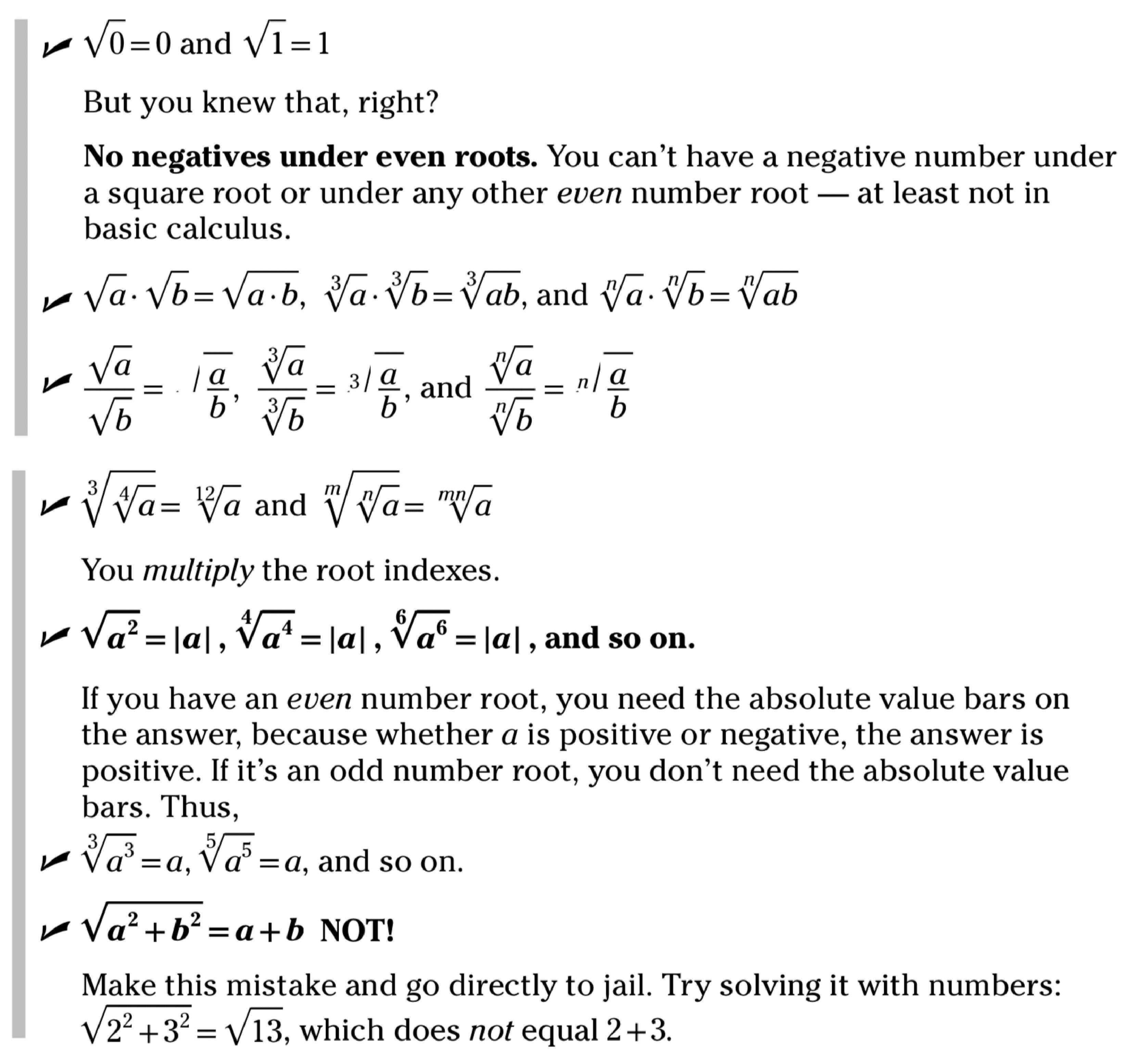
Properties of Roots
Taken from Calculus for Dummies

Properties of Logarithms
Taken from Calculus for Dummies
Finally, knowing how to solve quadratic equations can also come in handy in calculus.
If the quadratic equation is factorable, then the easiest method to solve it is to express the sum of terms in product form. For example, the following quadratic equation can be factored as follows:
x2 – 9 = (x + 3)(x – 3) = 0
Setting each factor to zero permits us to find a solution to this equation, which in this case is x = ±3.
Alternatively, the following quadratic formula may be used:
The Quadratic Formula
Taken from Calculus for Dummies
If we had to consider the same quadratic equation as above, then we would set the coefficient values to, a = 1, b = 0, and c = 9, which would again result in x = ±3 as our solution.
Fundamentals of Trigonometry
Trigonometry revolves around three main trigonometric functions, which are the sine, the cosine and the tangent, and their reciprocals, which are the cosecant, the secant and the cotangent, respectively.
When applied to a right angled triangle, these three main functions allow us to calculate the lengths of the sides, or any of the other two acute angles of the triangle, depending on the information that we have available to start off with. Specifically, for some angle, x, in the following 3-4-5 triangle:

The 3-4-5 Triangle
Taken from Calculus for Dummies
The Three Main Trigonometric Functions
Taken from Calculus for Dummies
The sine, cosine and tangent functions only work with right-angled triangles, and hence can only be used in the calculation of acute angles that are smaller than 90o. Nonetheless, if we had to work within the unit circle on the x–y coordinate plane, then we would be able to apply trigonometry to all angles between 0o and 360o:
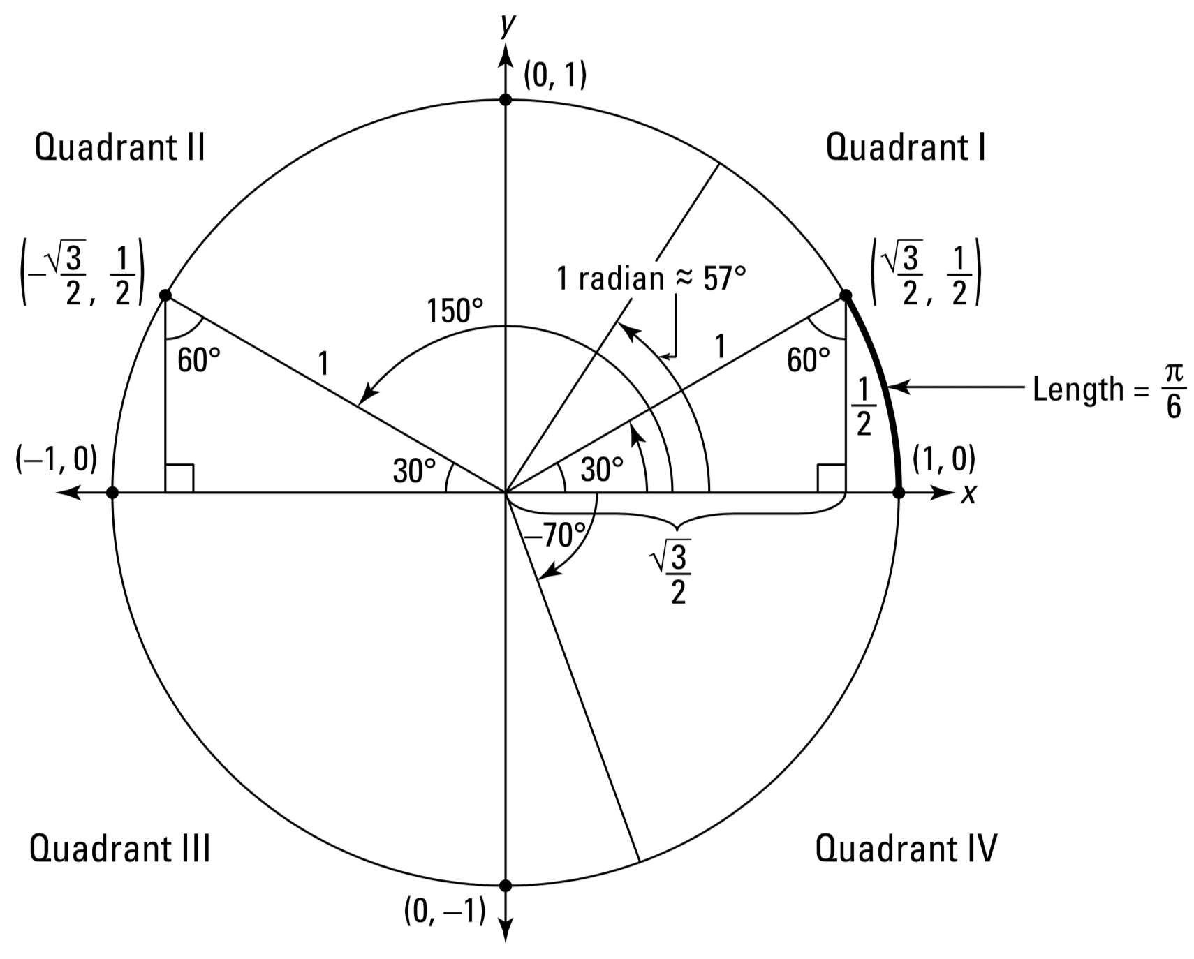
The Unit Circle
Taken from Calculus for Dummies
The unit circle has its center at the origin of the x–y coordinate plane, and a radius of one unit. Rotations around the unit circle are performed in a counterclockwise manner, starting from the positive x-axis. The cosine of the rotated angle would then be given by the x-coordinate of the point that hits the unit circle, whereas the y-coordinate specifies the sine of the rotated angle. It is also worth noting that the quadrants are symmetrical, and hence a point in one quadrant has symmetrical counterparts in the other three.
The graphed sine, cosine and tangent functions appear as follows:

Line Plots of the Sine, Cosine and Tangent Functions
Taken from Calculus for Dummies
All functions are periodic, with the sine and cosine functions featuring the same shape albeit being displaced by 90o between one another. The sine and cosine functions may, indeed, be easily sketched from the calculated x– and y-coordinates as one rotates around the unit circle. The tangent function may also be sketched similarly, since for any angle ???? this function may be defined by:
tan ???? = sin ???? / cos ???? = y / x
The tangent function is undefined at ±90o, since the cosine in the denominator returns a value of zero at this angle. Hence, we draw vertical asymptotes at these angles, which are imaginary lines that the curve approaches but never touches.
One final note concerns the inverse of these trigonometric functions. Taking the sine function as an example, its inverse is denoted by sin-1. This is not to be mistaken for the cosecant function, which is rather the reciprocal of sine, and hence not the same as its inverse.
Further Reading
This section provides more resources on the topic if you are looking to go deeper.
Books
- Deep Learning, 2019.
- Calculus for Dummies, 2016.
- The Hitchhiker’s Guide to Calculus, 2019.
Summary
In this tutorial, you discovered several pre-requisites for working with calculus.
Specifically, you learned:
- Linear and non-linear functions are central to calculus and machine learning, and many calculus problems involve their use.
- Fundamental concepts from algebra and trigonometry provide the foundations for calculus, and will become especially important as we tackle more advanced calculus topics.
Do you have any questions?
Ask your questions in the comments below and I will do my best to answer.
Get a Handle on Calculus for Machine Learning!
Feel Smarter with Calculus Concepts
...by getting a better sense on the calculus symbols and terms
Discover how in my new Ebook:
Calculus for Machine Learning
It provides self-study tutorials with full working code on:
differntiation, gradient, Lagrangian mutiplier approach, Jacobian matrix,
and much more...
")


Your Fractional Powers illustration is not correct: You need to swap a and b.
Indeed, thank you for pointing this out! This had escaped my proofreading.
Thank you very much Stefania; this is a beautiful article at a critical time in my academic/career path!