Calculus is one of the core mathematical concepts in machine learning that permits us to understand the internal workings of different machine learning algorithms.
One of the important applications of calculus in machine learning is the gradient descent algorithm, which, in tandem with backpropagation, allows us to train a neural network model.
In this tutorial, you will discover the integral role of calculus in machine learning.
After completing this tutorial, you will know:
- Calculus plays an integral role in understanding the internal workings of machine learning algorithms, such as the gradient descent algorithm for minimizing an error function.
- Calculus provides us with the necessary tools to optimise complex objective functions as well as functions with multidimensional inputs, which are representative of different machine learning applications.
Let’s get started.

Calculus in Machine Learning: Why it Works
Photo by Hasmik Ghazaryan Olson, some rights reserved.
Tutorial Overview
This tutorial is divided into two parts; they are:
- Calculus in Machine Learning
- Why Calculus in Machine Learning Works
Calculus in Machine Learning
A neural network model, whether shallow or deep, implements a function that maps a set of inputs to expected outputs.
The function implemented by the neural network is learned through a training process, which iteratively searches for a set of weights that best enable the neural network to model the variations in the training data.
A very simple type of function is a linear mapping from a single input to a single output.
Page 187, Deep Learning, 2019.
Such a linear function can be represented by the equation of a line having a slope, m, and a y-intercept, c:
y = mx + c
Varying each of parameters, m and c, produces different linear models that define different input-output mappings.

Line Plot of Different Line Models Produced by Varying the Slope and Intercept
Taken from Deep Learning
The process of learning the mapping function, therefore, involves the approximation of these model parameters, or weights, that result in the minimum error between the predicted and target outputs. This error is calculated by means of a loss function, cost function, or error function, as often used interchangeably, and the process of minimizing the loss is referred to as function optimization.
We can apply differential calculus to the process of function optimization.
In order to understand better how differential calculus can be applied to function optimization, let us return to our specific example of having a linear mapping function.
Say that we have some dataset of single input features, x, and their corresponding target outputs, y. In order to measure the error on the dataset, we shall be taking the sum of squared errors (SSE), computed between the predicted and target outputs, as our loss function.
Carrying out a parameter sweep across different values for the model weights, w0 = m and w1 = c, generates individual error profiles that are convex in shape.

Line Plots of Error (SSE) Profiles Generated When Sweeping Across a Range of Values for the Slope and Intercept
Taken from Deep Learning
Combining the individual error profiles generates a three-dimensional error surface that is also convex in shape. This error surface is contained within a weight space, which is defined by the swept ranges of values for the model weights, w0 and w1.
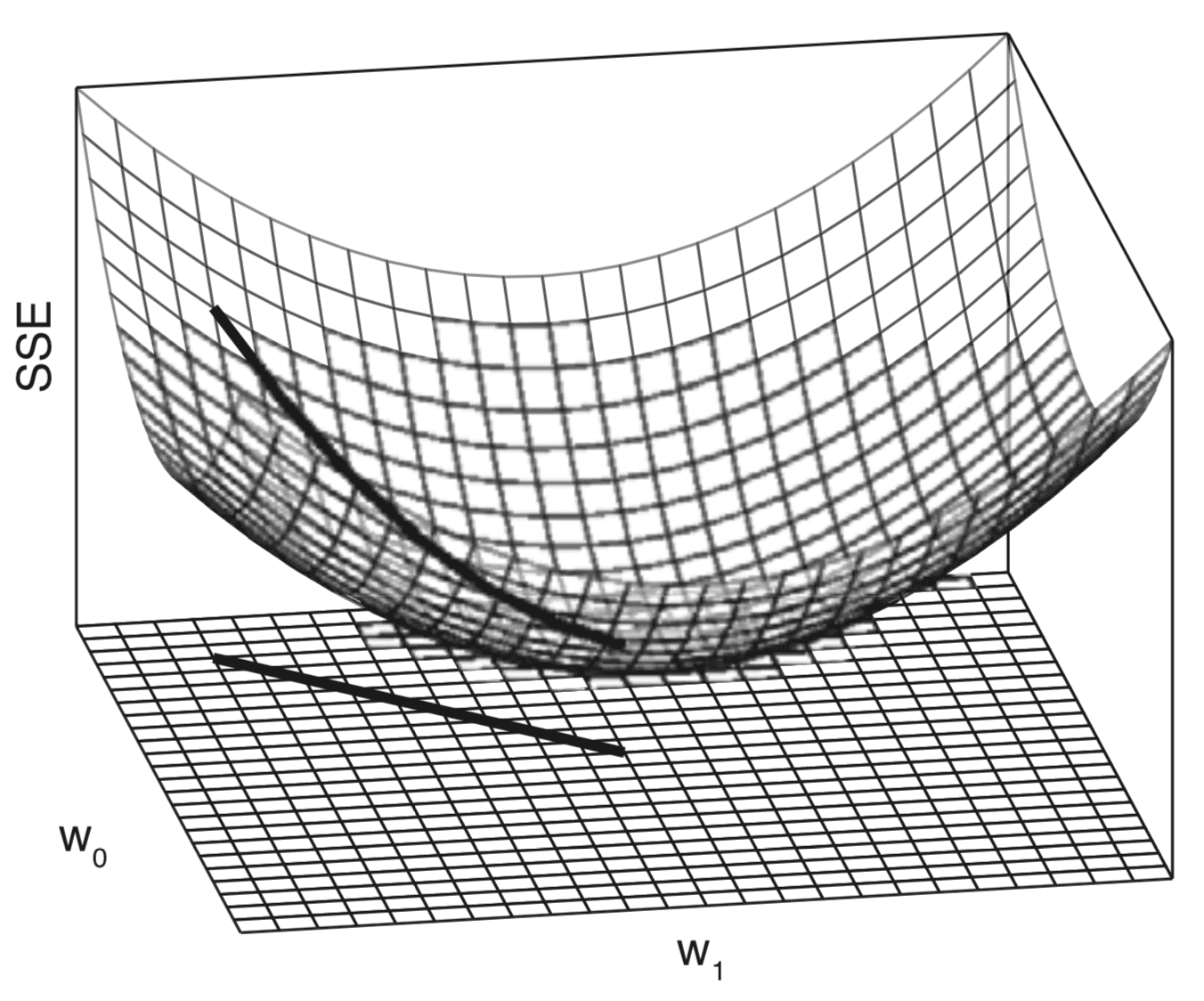
Three-Dimensional Plot of the Error (SSE) Surface Generated When Both Slope and Intercept are Varied
Taken from Deep Learning
Moving across this weight space is equivalent to moving between different linear models. Our objective is to identify the model that best fits the data among all possible alternatives. The best model is characterised by the lowest error on the dataset, which corresponds with the lowest point on the error surface.
A convex or bowl-shaped error surface is incredibly useful for learning a linear function to model a dataset because it means that the learning process can be framed as a search for the lowest point on the error surface. The standard algorithm used to find this lowest point is known as gradient descent.
Page 194, Deep Learning, 2019.
The gradient descent algorithm, as the optimization algorithm, will seek to reach the lowest point on the error surface by following its gradient downhill. This descent is based upon the computation of the gradient, or slope, of the error surface.
This is where differential calculus comes into the picture.
Calculus, and in particular differentiation, is the field of mathematics that deals with rates of change.
Page 198, Deep Learning, 2019.
More formally, let us denote the function that we would like to optimize by:
error = f(weights)
By computing the rate of change, or the slope, of the error with respect to the weights, the gradient descent algorithm can decide on how to change the weights in order to keep reducing the error.
Why Calculus in Machine Learning Works
The error function that we have considered to optimize is relatively simple, because it is convex and characterised by a single global minimum.
Nonetheless, in the context of machine learning, we often need to optimize more complex functions that can make the optimization task very challenging. Optimization can become even more challenging if the input to the function is also multidimensional.
Calculus provides us with the necessary tools to address both challenges.
Suppose that we have a more generic function that we wish to minimize, and which takes a real input, x, to produce a real output, y:
y = f(x)
Computing the rate of change at different values of x is useful because it gives us an indication of the changes that we need to apply to x, in order to obtain the corresponding changes in y.
Since we are minimizing the function, our goal is to reach a point that obtains as low a value of f(x) as possible that is also characterised by zero rate of change; hence, a global minimum. Depending on the complexity of the function, this may not necessarily be possible since there may be many local minima or saddle points that the optimisation algorithm may remain caught into.
In the context of deep learning, we optimize functions that may have many local minima that are not optimal, and many saddle points surrounded by very flat regions.
Page 84, Deep Learning, 2017.
Hence, within the context of deep learning, we often accept a suboptimal solution that may not necessarily correspond to a global minimum, so long as it corresponds to a very low value of f(x).

Line Plot of Cost Function to Minimize Displaying Local and Global Minima
Taken from Deep Learning
If the function we are working with takes multiple inputs, calculus also provides us with the concept of partial derivatives; or in simpler terms, a method to calculate the rate of change of y with respect to changes in each one of the inputs, xi, while holding the remaining inputs constant.
This is why each of the weights is updated independently in the gradient descent algorithm: the weight update rule is dependent on the partial derivative of the SSE for each weight, and because there is a different partial derivative for each weight, there is a separate weight update rule for each weight.
Page 200, Deep Learning, 2019.
Hence, if we consider again the minimization of an error function, calculating the partial derivative for the error with respect to each specific weight permits that each weight is updated independently of the others.
This also means that the gradient descent algorithm may not follow a straight path down the error surface. Rather, each weight will be updated in proportion to the local gradient of the error curve. Hence, one weight may be updated by a larger amount than another, as much as needed for the gradient descent algorithm to reach the function minimum.
Further Reading
This section provides more resources on the topic if you are looking to go deeper.
Books
- Deep Learning, 2019.
- Deep Learning, 2017.
Summary
In this tutorial, you discovered the integral role of calculus in machine learning.
Specifically, you learned:
- Calculus plays an integral role in understanding the internal workings of machine learning algorithms, such as the gradient descent algorithm that minimizes an error function based on the computation of the rate of change.
- The concept of the rate of change in calculus can also be exploited to minimise more complex objective functions that are not necessarily convex in shape.
- The calculation of the partial derivative, another important concept in calculus, permits us to work with functions that take multiple inputs.
Do you have any questions?
Ask your questions in the comments below and I will do my best to answer.
Get a Handle on Calculus for Machine Learning!
Feel Smarter with Calculus Concepts
...by getting a better sense on the calculus symbols and terms
Discover how in my new Ebook:
Calculus for Machine Learning
It provides self-study tutorials with full working code on:
differntiation, gradient, Lagrangian mutiplier approach, Jacobian matrix,
and much more...

")


Thanks for the tutorial.
When training DL/ML models with severals local optima how can i guarantee that the local optima found by the model is the lowest among them or the highest. and how can i overcome the situation when the model stuck and the hghest local optima.
Thanks/
Quoting from Pattern Recognition and Machine Learning, “For a successful application of neural networks, it may not be necessary to find the global minimum (and in general it will not be known whether the global minimum has been found) but it may be necessary to compare several local minima in order to find a sufficiently good solution.”
One way to do so is to monitor your model performance on a validation dataset (refer to this article), to stop training when the desired validation loss has been achieved. There are, also, different extensions to the gradient descent algorithm to control its behaviour downhill. I suggest that you write gradient descent in the search bar to see the different options.