The advance of generative machine learning models makes computers capable of creative work. In the scope of drawing pictures, there are a few notable models that allow you to convert a textual description into an array of pixels. The most powerful models today are part of the family of diffusion models. In this post, you will learn how this kind of model works and how you can control its output.
Kick-start your project with my book Mastering Digital Art with Stable Diffusion. It provides self-study tutorials with working code.
Let’s get started.
Brief Introduction to Diffusion Models for Image Generation
Photo by Dhruvin Pandya. Some rights reserved.
Overview
This post is in three parts; they are:
- Workflow of Diffusion Models
- Variation in Output
- How It was Trained
Workflow of Diffusion Models
Considering the goal of converting a description of a picture in text into a picture in an array of pixels, the machine learning model should have its output as an array of RGB values. But how should you provide text input to a model, and how is the conversion performed?
Since the text input describes the output, the model needs to understand what the text means. The better such a description is understood, the more accurate your model can generate the output. Hence, the trivial solution of treating the text as a character string does not work well. You need a module that can understand natural language, and the state-of-the-art solution would be to represent the input as embedding vectors.
Embedding representation of input text not only allows you to distill the meaning of the text but also provides a uniform shape of the input since the text of various lengths can be transformed into a standard size of tensors.
There are multiple ways to convert a tensor of the embedding representation into pixels. Recall how the generative adversarial network (GAN) works; you should notice this is in a similar structure, namely, the input (text) is converted into a latent structure (embedding), and then converted into the output (pixels).
Diffusion models are a family of neural network models that consider embedding to be a hint to restore a picture from random pixels. Below is a figure from the paper by Rombach et al. to illustrate this workflow:
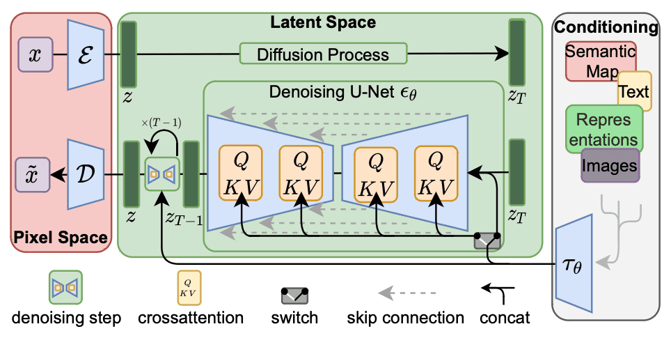
Stable Diffusion architecture. Figure from Rombach et al (2021)
In this figure, the workflow is from right to left. The output at the left is to convert a tensor into pixel space, using a decoder network denoted with $\mathcal{D}$. The input at the right is converted into an embedding $\tau_\theta$ which is used as the conditioning tensor. The key structure is in the latent space in the middle. The generation part is at the lower half of the green box, which converts $z_T$ into $z_{T-1}$ using a denoising network $\epsilon_\theta$.
The denoising network takes an input tensor $z_T$ and the embedding $\tau_\theta$, outputs a tensor $z_{T-1}$. The output is a tensor that is “better” than the input in the sense that it matches better to the embedding. In its simplest form, the decoder $\mathcal{D}$ does nothing but copy over the output from the latent space. The input and output tensors $z_T$ and $z_{T-1}$ of the denoising network are arrays of RGB pixels, which the network make it less noisy.
It is called the denoising network because it assumes the embedding can describe the output perfectly, but the input and the output differ because some pixels are replaced by random values. The network model aimed at removing such random values and restoring the original pixel. It is a difficult task, but the model assumes the noise pixels are added uniformly, and the noise follows a Gaussian model. Hence, the model can be reused many times, each producing an improvement in the input. Below is an illustration from the paper by Ho et al. for such a concept:
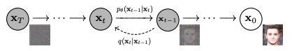
Denoising an image. Figure from Ho et al. (2020)
Because of this structure, the denoising network assumes the input $z_T$ and output $z_{T-1}$ are in the same shape, such that the network can be repeated until the final output $z$ is produced. The denoising U-net block in the previous figure is to keep the input and output of the same shape. The denoising block conceptually is to perform the following:
$$
\begin{aligned}
w_t &= \textrm{NoisePredictor}(z_t, \tau_\theta, t) \\
z_{t-1} &= z_t – w_t
\end{aligned}
$$
that is, the noise component $w_t$ is predicted from the noisy image $z_t$, the conditioning tensor $\tau_\theta$, and the step count $t$. The noise predictor then based on $t$ to estimate the level of noise in $z_t$ conditioned on the what the final image $z=z_0$ should be as described by the tensor $\tau_theta$. The value of $t$ is helpful to the predictor because the larger the value, the more noise it is in $z_t$.
Subtracting the noise from $z_t$ will be the denoised image $z_{t-1}$, which can be feed into the denoising network again until $z=z_0$ is produced. The number of times $T$ this network processed the tensor is a design parameter to the entire diffusion model. Because in this model, the noise is formulated as Gaussian, a part of the decoder $\mathcal{D}$ is to convert the latent space tensor $z$ into a three-channel tensor and quantize floating point values into RGB.
Variation in Output
Once the neural network is trained, the weights in each layer are fixed, and the output is deterministic as long as the input is deterministic. However, in this diffusion model workflow, the input is the text that will be converted into embedding vectors. The denoising model takes an additional input, the initial $z_T$ tensor in the latent space. This is usually generated randomly, such as by sampling a Gaussian distribution and filling in the tensor of the shape that the denoising network expects. With a different starting tensor, you get a different output. This is how you can generate different output by the same input text.
Indeed, the reality is much more complicated than this. Remember that the denoising network is run in multiple steps, each step aimed at improving the output a bit until the pristine final output is produced. The network can take an additional hint of which step it is in (e.g., step 5 of a total of 10 steps scheduled). Gaussian noise is parameterized by its mean and variation, which you can provide a function to calculate. The better you can model the noise expected at each step, the better the denoising network can remove the noise. In the Stable Diffusion model, the denoising network needs a sample of random noise reflecting the noise intensity as in that step to predict the noise component from an noisy image. Algorithm 2 in the figure below shows this, which such randomness is introduced as $\sigma_t\mathbf{z}$. You can select the sampler for such a purpose. Some samplers converge faster than others (i.e., you use fewer steps). You can also consider the latent space model as a variation autoencoder, in which the variations introduced affect the output as well.
How It Was Trained
Taking the Stable Diffusion model as an example, you can see that the most important component in the workflow is the denosing model in the latent space. Indeed, the input model is not trained but adopts an existing text embedding model, such as BERT or T5. The output model can also be an off-the-shelf model, such as a super-resolution model that converts a 256×256 pixel image into a 512×512 pixel image.
Training the denoising network model conceptually is as follows: You pick an image and add some noise to it. Then you created a tuple of three components: The image, the noise, and the noisy image. The network is then trained to estimate the noise part of the noisy image. The noise part can vary by different weight of adding noise to the pixels, as well as the Gaussian parameters to generate the noise. The training algorithm is depicted in Algorithm 1 as follows:
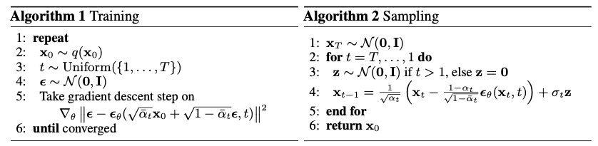
Training and sampling algorithms. Figure from Ho et al (2020)
Since the denoising network assumes the noise is additive, the noise predicted can be subtracted from the input to produce the output. As described above, the denoising network takes not only the image as the input but also the embedding that reflects the text input. The embedding plays a role in that the noise to detect is conditioned to the embedding, which means the output should related to the embedding, and the noise to detect should fit a conditional probability distribution. Technically, the image and the embedding meet each other using a cross-attention mechanism in the latent model, which is not shown in the skeleton of algorithms above.
There is a lot of vocabulary to describe a picture, and you can imagine it is not easy to make the network model learn how to correlate a word to a picture. It is reported that Stable Diffusion model, for example, was trained with 2.3 billion images and consumed 150 thousand GPU hours, using the LAION-5B dataset (which has 5.85 billion images with text descriptions). However, once the model is trained, you can use it on a commodity computer such as your laptop.
Further Readings
Below are several papers that created the diffusion models for image generation as we know it today:
- “High-Resolution Image Synthesis with Latent Diffusion Models” by Rombach, Blattmann, Lorenz, Esser, and Ommer (2021)
arXiv 2112.10752 - “Denoising Diffusion Probabilistic Models” by Ho, Jain, and Abbeel (2020)
arXiv 2006.11239 - “Diffusion Models Beat GANs on Image Synthesis” by Dhariwal and Nichol (2021)
arXiv 2105.05233 - “Improved Denoising Diffusion Probabilistic Models” by Nichol and Dhariwal (2021)
arXiv 2102.09672
Summary
In this post, you saw an overview of how a diffusion model works. In particular, you learned
- The image generation workflow has multiple steps, the diffusion model works at the latent space as a denoising neural network.
- Image generation is achieved by starting from a noisy image, which is an array of randomly generated pixels.
- In each step in the latent space, the denoising network removes some noise, conditioned to the input text description of the final image in the form of embedding vectors.
- The output image is obtained by decoding the output from the latent space.
Get Started on Mastering Digital Art with Stable Diffusion!

Learn how to make Stable Diffusion work for you
...by learning some key elements in the image generation process
Discover how in my new Ebook:
Mastering Digital Art with Stable Diffusion
This book offers self-study tutorials complete with all the working code in Python, guiding you from a novice to an expert in image generation. It teaches you how to set up Stable Diffusion, fine-tune models, automate workflows, adjust key parameters, and much more...all to help you create stunning digital art.


No comments yet.