The gradient descent algorithm is one of the most popular techniques for training deep neural networks. It has many applications in fields such as computer vision, speech recognition, and natural language processing. While the idea of gradient descent has been around for decades, it’s only recently that it’s been applied to applications related to deep learning.
Gradient descent is an iterative optimization method used to find the minimum of an objective function by updating values iteratively on each step. With each iteration, it takes small steps towards the desired direction until convergence, or a stop criterion is met.
In this tutorial, you will train a simple linear regression model with two trainable parameters and explore how gradient descent works and how to implement it in PyTorch. Particularly, you’ll learn about:
- Gradient Descent algorithm and its implementation in PyTorch
- Batch Gradient Descent and its implementation in PyTorch
- Stochastic Gradient Descent and its implementation in PyTorch
- How Batch Gradient Descent and Stochastic Gradient Descent are different from each other
- How loss decreases in Batch Gradient Descent and Stochastic Gradient Descent during training
Kick-start your project with my book Deep Learning with PyTorch. It provides self-study tutorials with working code.
So, let’s get started.
Implementing Gradient Descent in PyTorch.
Picture by Michael Behrens. Some rights reserved.
Overview
This tutorial is in four parts; they are
- Preparing Data
- Batch Gradient Descent
- Stochastic Gradient Descent
- Plotting Graphs for Comparison
Preparing Data
To keep the model simple for illustration, we will use the linear regression problem as in the last tutorial. The data is synthetic and generated as follows:
|
1 2 3 4 5 6 7 8 9 10 |
import torch import numpy as np import matplotlib.pyplot as plt # Creating a function f(X) with a slope of -5 X = torch.arange(-5, 5, 0.1).view(-1, 1) func = -5 * X # Adding Gaussian noise to the function f(X) and saving it in Y Y = func + 0.4 * torch.randn(X.size()) |
Same as in the previous tutorial, we initialized a variable X with values ranging from $-5$ to $5$, and created a linear function with a slope of $-5$. Then, Gaussian noise is added to create the variable Y.
We can plot the data using matplotlib to visualize the pattern:
|
1 2 3 4 5 6 7 8 9 |
... # Plot and visualizing the data points in blue plt.plot(X.numpy(), Y.numpy(), 'b+', label='Y') plt.plot(X.numpy(), func.numpy(), 'r', label='func') plt.xlabel('x') plt.ylabel('y') plt.legend() plt.grid('True', color='y') plt.show() |
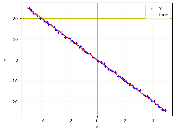
Data points for regression model
Want to Get Started With Deep Learning with PyTorch?
Take my free email crash course now (with sample code).
Click to sign-up and also get a free PDF Ebook version of the course.
Batch Gradient Descent
Now that we have created the data for our model, next we’ll build a forward function based on a simple linear regression equation. We’ll train the model for two parameters ($w$ and $b$). We will also need a loss criterion function. Because it is a regression problem on continuous values, MSE loss is appropriate.
|
1 2 3 4 5 6 7 8 |
... # defining the function for forward pass for prediction def forward(x): return w * x + b # evaluating data points with Mean Square Error (MSE) def criterion(y_pred, y): return torch.mean((y_pred - y) ** 2) |
Before we train our model, let’s learn about the batch gradient descent. In batch gradient descent, all the samples in the training data are considered in a single step. The parameters are updated by taking the mean gradient of all the training examples. In other words, there is only one step of gradient descent in one epoch.
While Batch Gradient Descent is the best choice for smooth error manifolds, it’s relatively slow and computationally complex, especially if you have a larger dataset for training.
Training with Batch Gradient Descent
Let’s randomly initialize the trainable parameters $w$ and $b$, and define some training parameters such as learning rate or step size, an empty list to store the loss, and number of epochs for training.
|
1 2 3 4 5 6 |
w = torch.tensor(-10.0, requires_grad=True) b = torch.tensor(-20.0, requires_grad=True) step_size = 0.1 loss_BGD = [] n_iter = 20 |
We’ll train our model for 20 epochs using below lines of code. Here, the forward() function generates the prediction while the criterion() function measures the loss to store it in loss variable. The backward() method performs the gradient computations and the updated parameters are stored in w.data and b.data.
|
1 2 3 4 5 6 7 8 9 10 11 12 13 14 15 16 17 |
for i in range (n_iter): # making predictions with forward pass Y_pred = forward(X) # calculating the loss between original and predicted data points loss = criterion(Y_pred, Y) # storing the calculated loss in a list loss_BGD.append(loss.item()) # backward pass for computing the gradients of the loss w.r.t to learnable parameters loss.backward() # updateing the parameters after each iteration w.data = w.data - step_size * w.grad.data b.data = b.data - step_size * b.grad.data # zeroing gradients after each iteration w.grad.data.zero_() b.grad.data.zero_() # priting the values for understanding print('{}, \t{}, \t{}, \t{}'.format(i, loss.item(), w.item(), b.item())) |
Here is the how the output looks like and the parameters are updated after every epoch when we apply batch gradient descent.
|
1 2 3 4 5 6 7 8 9 10 11 12 13 14 15 16 17 18 19 20 |
0, 596.7191162109375, -1.8527469635009766, -16.062074661254883 1, 343.426513671875, -7.247585773468018, -12.83026123046875 2, 202.7098388671875, -3.616910219192505, -10.298759460449219 3, 122.16651153564453, -6.0132551193237305, -8.237251281738281 4, 74.85094451904297, -4.394278526306152, -6.6120076179504395 5, 46.450958251953125, -5.457883358001709, -5.295622825622559 6, 29.111614227294922, -4.735295295715332, -4.2531514167785645 7, 18.386211395263672, -5.206836700439453, -3.4119482040405273 8, 11.687058448791504, -4.883906364440918, -2.7437009811401367 9, 7.4728569984436035, -5.092618465423584, -2.205873966217041 10, 4.808231830596924, -4.948029518127441, -1.777699589729309 11, 3.1172332763671875, -5.040188312530518, -1.4337140321731567 12, 2.0413269996643066, -4.975278854370117, -1.159447193145752 13, 1.355530858039856, -5.0158305168151855, -0.9393846988677979 14, 0.9178376793861389, -4.986582279205322, -0.7637402415275574 15, 0.6382412910461426, -5.004333972930908, -0.6229321360588074 16, 0.45952412486076355, -4.991086006164551, -0.5104631781578064 17, 0.34523946046829224, -4.998797416687012, -0.42035552859306335 18, 0.27213525772094727, -4.992753028869629, -0.3483465909957886 19, 0.22536347806453705, -4.996064186096191, -0.2906789183616638 |
Putting all together, the following is the complete code
|
1 2 3 4 5 6 7 8 9 10 11 12 13 14 15 16 17 18 19 20 21 22 23 24 25 26 27 28 29 30 31 32 33 34 35 36 37 38 39 40 |
import torch import numpy as np import matplotlib.pyplot as plt X = torch.arange(-5, 5, 0.1).view(-1, 1) func = -5 * X Y = func + 0.4 * torch.randn(X.size()) # defining the function for forward pass for prediction def forward(x): return w * x + b # evaluating data points with Mean Square Error (MSE) def criterion(y_pred, y): return torch.mean((y_pred - y) ** 2) w = torch.tensor(-10.0, requires_grad=True) b = torch.tensor(-20.0, requires_grad=True) step_size = 0.1 loss_BGD = [] n_iter = 20 for i in range (n_iter): # making predictions with forward pass Y_pred = forward(X) # calculating the loss between original and predicted data points loss = criterion(Y_pred, Y) # storing the calculated loss in a list loss_BGD.append(loss.item()) # backward pass for computing the gradients of the loss w.r.t to learnable parameters loss.backward() # updateing the parameters after each iteration w.data = w.data - step_size * w.grad.data b.data = b.data - step_size * b.grad.data # zeroing gradients after each iteration w.grad.data.zero_() b.grad.data.zero_() # priting the values for understanding print('{}, \t{}, \t{}, \t{}'.format(i, loss.item(), w.item(), b.item())) |
The for-loop above prints one line per epoch, such as the following:
|
1 2 3 4 5 6 7 8 9 10 11 12 13 14 15 16 17 18 19 20 |
0, 596.7191162109375, -1.8527469635009766, -16.062074661254883 1, 343.426513671875, -7.247585773468018, -12.83026123046875 2, 202.7098388671875, -3.616910219192505, -10.298759460449219 3, 122.16651153564453, -6.0132551193237305, -8.237251281738281 4, 74.85094451904297, -4.394278526306152, -6.6120076179504395 5, 46.450958251953125, -5.457883358001709, -5.295622825622559 6, 29.111614227294922, -4.735295295715332, -4.2531514167785645 7, 18.386211395263672, -5.206836700439453, -3.4119482040405273 8, 11.687058448791504, -4.883906364440918, -2.7437009811401367 9, 7.4728569984436035, -5.092618465423584, -2.205873966217041 10, 4.808231830596924, -4.948029518127441, -1.777699589729309 11, 3.1172332763671875, -5.040188312530518, -1.4337140321731567 12, 2.0413269996643066, -4.975278854370117, -1.159447193145752 13, 1.355530858039856, -5.0158305168151855, -0.9393846988677979 14, 0.9178376793861389, -4.986582279205322, -0.7637402415275574 15, 0.6382412910461426, -5.004333972930908, -0.6229321360588074 16, 0.45952412486076355, -4.991086006164551, -0.5104631781578064 17, 0.34523946046829224, -4.998797416687012, -0.42035552859306335 18, 0.27213525772094727, -4.992753028869629, -0.3483465909957886 19, 0.22536347806453705, -4.996064186096191, -0.2906789183616638 |
Stochastic Gradient Descent
As we learned that batch gradient descent is not a suitable choice when it comes to a huge training data. However, deep learning algorithms are data hungry and often require large quantity of data for training. For instance, a dataset with millions of training examples would require the model to compute the gradient for all data in a single step, if we are using batch gradient descent.
This doesn’t seem to be an efficient way and the alternative is stochastic gradient descent (SGD). Stochastic gradient descent considers only a single sample from the training data at a time, computes the gradient to take a step, and update the weights. Therefore, if we have $N$ samples in the training data, there will be $N$ steps in each epoch.
Training with Stochastic Gradient Descent
To train our model with stochastic gradient descent, we’ll randomly initialize the trainable parameters $w$ and $b$ as we did for the batch gradient descent above. Here we’ll define an empty list to store the loss for stochastic gradient descent and train the model for 20 epochs. The following is the complete code modified from the previous example:
|
1 2 3 4 5 6 7 8 9 10 11 12 13 14 15 16 17 18 19 20 21 22 23 24 25 26 27 28 29 30 31 32 33 34 35 36 37 38 39 40 41 42 43 44 |
import torch import numpy as np import matplotlib.pyplot as plt X = torch.arange(-5, 5, 0.1).view(-1, 1) func = -5 * X Y = func + 0.4 * torch.randn(X.size()) # defining the function for forward pass for prediction def forward(x): return w * x + b # evaluating data points with Mean Square Error (MSE) def criterion(y_pred, y): return torch.mean((y_pred - y) ** 2) w = torch.tensor(-10.0, requires_grad=True) b = torch.tensor(-20.0, requires_grad=True) step_size = 0.1 loss_SGD = [] n_iter = 20 for i in range (n_iter): # calculating true loss and storing it Y_pred = forward(X) # store the loss in the list loss_SGD.append(criterion(Y_pred, Y).tolist()) for x, y in zip(X, Y): # making a pridiction in forward pass y_hat = forward(x) # calculating the loss between original and predicted data points loss = criterion(y_hat, y) # backward pass for computing the gradients of the loss w.r.t to learnable parameters loss.backward() # updateing the parameters after each iteration w.data = w.data - step_size * w.grad.data b.data = b.data - step_size * b.grad.data # zeroing gradients after each iteration w.grad.data.zero_() b.grad.data.zero_() # priting the values for understanding print('{}, \t{}, \t{}, \t{}'.format(i, loss.item(), w.item(), b.item())) |
This prints a long list of values as follows
|
1 2 3 4 5 6 7 8 9 |
0, 24.73763084411621, -5.02630615234375, -20.994739532470703 0, 455.0946960449219, -25.93259620666504, -16.7281494140625 0, 6968.82666015625, 54.207733154296875, -33.424049377441406 0, 97112.9140625, -238.72393798828125, 28.901844024658203 .... 19, 8858971136.0, -1976796.625, 8770213.0 19, 271135948800.0, -1487331.875, 8874354.0 19, 3010866446336.0, -3153109.5, 8527317.0 19, 47926483091456.0, 3631328.0, 9911896.0 |
Plotting Graphs for Comparison
Now that we have trained our model using batch gradient descent and stochastic gradient descent, let’s visualize how the loss decreases for both the methods during model training. So, the graph for batch gradient descent looks like this.
|
1 2 3 4 5 6 |
... plt.plot(loss_BGD, label="Batch Gradient Descent") plt.xlabel('Epoch') plt.ylabel('Cost/Total loss') plt.legend() plt.show() |
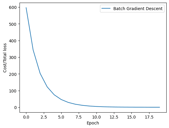
The loss history of batch gradient descent
Similarly, here is how the graph for stochastic gradient descent looks like.
|
1 2 3 4 5 |
plt.plot(loss_SGD,label="Stochastic Gradient Descent") plt.xlabel('Epoch') plt.ylabel('Cost/Total loss') plt.legend() plt.show() |
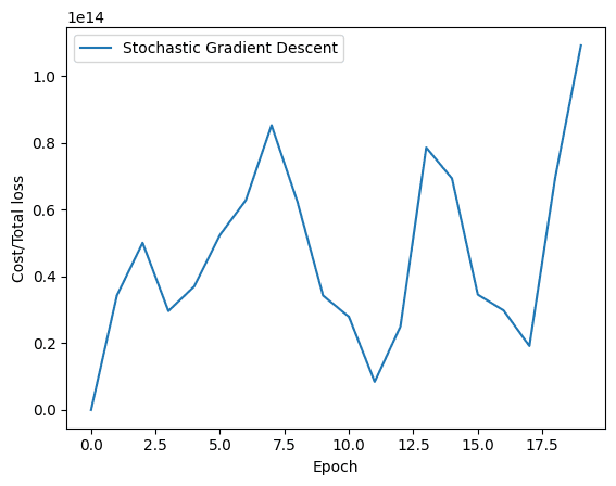
Loss history of stochastic gradient descent
As you can see, the loss smoothly decreases for batch gradient descent. On the other hand, you’ll observe fluctuations in the graph for stochastic gradient descent. As mentioned earlier, the reason is quite simple. In batch gradient descent, the loss is updated after all the training samples are processed while the stochastic gradient descent updates the loss after every training sample in the training data.
Putting everything together, below is the complete code:
|
1 2 3 4 5 6 7 8 9 10 11 12 13 14 15 16 17 18 19 20 21 22 23 24 25 26 27 28 29 30 31 32 33 34 35 36 37 38 39 40 41 42 43 44 45 46 47 48 49 50 51 52 53 54 55 56 57 58 59 60 61 62 63 64 65 66 67 68 69 70 71 72 73 74 75 76 77 78 79 80 81 82 83 84 85 86 87 88 89 90 91 92 93 94 |
import torch import numpy as np import matplotlib.pyplot as plt # Creating a function f(X) with a slope of -5 X = torch.arange(-5, 5, 0.1).view(-1, 1) func = -5 * X # Adding Gaussian noise to the function f(X) and saving it in Y Y = func + 0.4 * torch.randn(X.size()) # Plot and visualizing the data points in blue plt.plot(X.numpy(), Y.numpy(), 'b+', label='Y') plt.plot(X.numpy(), func.numpy(), 'r', label='func') plt.xlabel('x') plt.ylabel('y') plt.legend() plt.grid('True', color='y') plt.show() # defining the function for forward pass for prediction def forward(x): return w * x + b # evaluating data points with Mean Square Error (MSE) def criterion(y_pred, y): return torch.mean((y_pred - y) ** 2) # Batch gradient descent w = torch.tensor(-10.0, requires_grad=True) b = torch.tensor(-20.0, requires_grad=True) step_size = 0.1 loss_BGD = [] n_iter = 20 for i in range (n_iter): # making predictions with forward pass Y_pred = forward(X) # calculating the loss between original and predicted data points loss = criterion(Y_pred, Y) # storing the calculated loss in a list loss_BGD.append(loss.item()) # backward pass for computing the gradients of the loss w.r.t to learnable parameters loss.backward() # updateing the parameters after each iteration w.data = w.data - step_size * w.grad.data b.data = b.data - step_size * b.grad.data # zeroing gradients after each iteration w.grad.data.zero_() b.grad.data.zero_() # priting the values for understanding print('{}, \t{}, \t{}, \t{}'.format(i, loss.item(), w.item(), b.item())) # Stochastic gradient descent w = torch.tensor(-10.0, requires_grad=True) b = torch.tensor(-20.0, requires_grad=True) step_size = 0.1 loss_SGD = [] n_iter = 20 for i in range(n_iter): # calculating true loss and storing it Y_pred = forward(X) # store the loss in the list loss_SGD.append(criterion(Y_pred, Y).tolist()) for x, y in zip(X, Y): # making a pridiction in forward pass y_hat = forward(x) # calculating the loss between original and predicted data points loss = criterion(y_hat, y) # backward pass for computing the gradients of the loss w.r.t to learnable parameters loss.backward() # updateing the parameters after each iteration w.data = w.data - step_size * w.grad.data b.data = b.data - step_size * b.grad.data # zeroing gradients after each iteration w.grad.data.zero_() b.grad.data.zero_() # priting the values for understanding print('{}, \t{}, \t{}, \t{}'.format(i, loss.item(), w.item(), b.item())) # Plot graphs plt.plot(loss_BGD, label="Batch Gradient Descent") plt.xlabel('Epoch') plt.ylabel('Cost/Total loss') plt.legend() plt.show() plt.plot(loss_SGD,label="Stochastic Gradient Descent") plt.xlabel('Epoch') plt.ylabel('Cost/Total loss') plt.legend() plt.show() |
Summary
In this tutorial you learned about the Gradient Descent, some of its variations, and how to implement them in PyTorch. Particularly, you learned about:
- Gradient Descent algorithm and its implementation in PyTorch
- Batch Gradient Descent and its implementation in PyTorch
- Stochastic Gradient Descent and its implementation in PyTorch
- How Batch Gradient Descent and Stochastic Gradient Descent are different from each other
- How loss decreases in Batch Gradient Descent and Stochastic Gradient Descent during training
Get Started on Deep Learning with PyTorch!

Learn how to build deep learning models
...using the newly released PyTorch 2.0 library
Discover how in my new Ebook:
Deep Learning with PyTorch
It provides self-study tutorials with hundreds of working code to turn you from a novice to expert. It equips you with
tensor operation, training, evaluation, hyperparameter optimization,
and much more...


Thank you for this code, it was quite helpful in my study. Unfortunately, SGD does not work.
But I suggest couple of corrections:
1) Just to beautify in 10th line: Y = func + torch.randn(X.size())
2) To make SGD works (here it is not convergent): step_size=0.001 for SGD only
3) To make SGD fits it description in wiki, make data shuffle before each epoch:
by adding before internal cycle
idx = torch.randperm(Y.shape[0])
X = X[idx].view(X.size())
Y = Y[idx].view(Y.size())
Hi Evgeny…You are very welcome! Please elaborate on why SGD is not sufficient for your model.
You may wish to try Adam:
https://machinelearningmastery.com/adam-optimization-algorithm-for-deep-learning/
It’s pretty far-fetched to use stochastic gradient descent for a linear regression problem, which admits a closed form solution… Why not doing it with another simple problem, like to logistic regression for instance?